Data Modeling Techniques

There are 3 major modeling approaches:

1️⃣ ER Model (Entity Relationship Model)

The Entity Relationship (ER) Model is a conceptual way of designing databases using:

Entities
Attributes
Relationships

Created by: Peter Chen

Traditional OLTP systems
Used in normalized databases

Used in:

Banking systems
Transactional systems

2️⃣ Dimensional Modeling

Dimensional Modeling is a data design technique used in Data Warehousing to support:

Reporting
BI tools
Analytics
Fast query performance

It was popularized by
Ralph Kimball.

👉 It is optimized for read performance, not transactions.

Created by: Ralph Kimball

Used in:

Data Warehousing
BI systems
Reporting

Used in:

Enterprise Data Warehouse
Power BI
Tableau
Snowflake / Teradata DW

⭐ Two main types:

🔹 Star Schema

A Star Schema is a dimensional model where:

One central Fact table
Multiple Denormalized Dimension tables
Structure looks like a ⭐ (star)

Both Star and Snowflake schemas are used in data warehouse design to organize and optimize data for reporting, analytics, and BI tools. They revolve around fact tables (numerical data) and dimension tables (descriptive data).

📌 Characteristics

✔ Dimensions are denormalized
✔ Fewer joins
✔ High query performance
✔ Easy to understand
✔ Best for BI tools

🧱 Structure

Example: Loan Analytics

🧠 Example

Fact_Loan

Loan_Key
Customer_Key
Channel_Key
Date_Key
Loan_Amount

Dim_Customer

Customer_Key
Name
City
Segment

All customer info in one table.

✔ Fast queries
✔ Easy reporting
✔ Best for Power BI / Tableau

🎯 Advantages

Fast aggregation queries
Simple design
Easy reporting
Better performance

❌ Disadvantages

Data redundancy in dimensions
Larger storage

🔹Snowflake Schema

A Snowflake Schema is a dimensional model where:

Fact table in center
Dimension tables are normalized
Looks like a snowflake ❄

Normalized dimensions
More joins
Less redundancy

📌 Characteristics

✔ Dimensions are normalized
✔ More joins
✔ Less redundancy
✔ Slightly complex

🎯 Advantages

Reduced storage
Better data consistency
Less duplication

❌ Disadvantages

More joins → Slower queries
Complex for BI tools
Harder to maintain

3️⃣ Data Vault Modeling

Data Vault is a data modeling methodology used in data warehousing to provide flexible, scalable, and audit-compliant solutions for storing historical enterprise data.

Data Vault is a data warehouse modeling technique designed for:

Scalability
Auditability
Historical tracking
Agile development

It was created by
Dan Linstedt.

👉 It solves limitations of traditional dimensional modeling in large enterprise systems.

✅ Why use Data Vault?

It handles rapidly changing data with traceability.
Great for agile development, big data, and real-time analytics.
Makes data warehouses more adaptable to business and structural changes.
Emphasizes auditing, historical tracking, and parallel loading.

Used in:

Enterprise Data Warehouse
Large scalable systems
Audit tracking
Agile data warehouse

🎯 Why Data Vault?

Traditional Star Schema problems:

Hard to adapt to new sources
Difficult schema changes
Limited audit tracking
Complex reprocessing

Data Vault solves this by:

✔ Separating business keys
✔ Storing history automatically
✔ Making it source-system friendly
✔ Supporting parallel loading

1️⃣ Hub

A Hub stores unique business keys — the identifiers that define a business entity regardless of which source system provides them.

Each hub represents a core business concept, such as they represent Customer Id/Product Number/Vehicle identification number (VIN).

Stores:

Business Key (natural key)
Load Date
Record Source
Hash Key (usually)

Hubs are immutable. Once a business key is loaded, it never changes.

Example:

Hub_Customer

Customer_HK (Hash Key)
Customer_ID (Business Key)
Load_Date
Record_Source

✔ One hub per business entity
✔ No descriptive attributes

2️⃣ Link

A Link stores relationships between Hubs.

Every relationship — customer-to-order, order-to-product, employee-to-department — gets its own Link table.

Stores:

Relationship between hubs

Links are also immutable. Once a relationship is recorded, it stays.

Links support many-to-many relationships by default. They answer the question: How are business concepts related?

Example:

Link_Loan_Customer

Loan_HK
Customer_HK
Load_Date
Record_Source

✔ Handles M:M relationships
✔ Only keys, no descriptions

3️⃣ Satellite

Satellites store the descriptive attributes of a Hub or Link, along with their change history.

Satellites fill the gap in answering the missing descriptive information on core business concepts. Satellites store information that belongs to Hub and relationships between them.

Stores:

Descriptive attributes
Historical changes
Effective dates

Every time an attribute changes, a new Satellite row is inserted. This is equivalent to SCD Type 2 — full history is preserved without modifying existing rows.

Different source systems can feed different Satellites for the same Hub, allowing attributes to arrive independently.

Example:

Sat_Customer_Details

Customer_HK
Name
Address
Phone
Load_Date
End_Date

✔ Keeps full history
✔ Insert-only model

👉 Data Vault is usually raw layer
👉 Star schema is presentation layer

🔥 Why Enterprises Prefer Data Vault

✔ Multiple source integration
✔ Regulatory compliance
✔ Audit requirement
✔ Banking / Finance systems
✔ Large-scale DW

✅ Comparison (Very Important)

Model	Used In	Pros	Cons
ER	OLTP	Highly normalized	Complex joins
Star	BI / Reporting	Fast queries	Data redundancy
Snowflake	BI	Less redundancy	More joins
Data Vault	Enterprise DW	Scalable & Auditable	Complex design

4️⃣ Multi Active Satellites

A Multi-Active Satellite (MAS) is a special type of satellite used in Data Vault modeling when multiple active records exist for the same business key and timestamp. This often happens when different versions of valid data co-exist simultaneously, not just sequentially over time.
for example, a customer has multiple active phone numbers or addresses concurrently.

5️⃣ Point-in-Time (PIT) Tables

Point In Time (PIT) tables in Data Vault modeling are specialized helper tables designed to simplify and optimize querying historical data that comes from multiple satellites related to a single hub or link. They are commonly used in Data Vault 2.0 implementations to improve query performance and reduce complexity.

🧠 Purpose of PIT Tables
In a Data Vault model:
- Hubs and satellites are normalized (efficient for storage and history).
- But querying them (especially time-based joins) is complex and slow.
- PIT tables provide a denormalized snapshot of satellite records for a specific time point.
🔁 This avoids repeated complex joins every time someone wants to get the data “as of” a specific date.
🧱 Structure of a PIT Table
A PIT table usually includes:

Business key hash (Hub Hash Key)
Load dates from multiple satellites
Optionally, a snapshot date (cutoff or PIT timestamp)

========================================================================

Entity-Relationship

ER Model is a conceptual framework used for designing and representing the logical structure of a database. It visually outlines entities, their attributes, and the relationships among them.

Entity in DBMS

An Entity is a real-world object, concept, or thing about which data is stored in a database.

In relational databases, entities are represented as tables, and individual entities are represented as rows.

Examples of Entities:

Objects: Employee, Car, Student
Concepts: Course, Event, Reservation
Things: Product, Document, Device

Entity Set

An Entity Set is a collection of similar types of entities (i.e., all rows in a table).
For example, all students in a university form the Student entity set.

⚠️ ER Diagrams represent entity sets, not individual entities.

What are Attributes?

Attributes are properties or characteristics of an entity that describe its details.

📌 Example: For a Student entity, attributes include Roll_No, Name, DOB, Address, etc.

In ER diagrams, attributes are represented by ovals.

Relationship Type and Relationship Set

A Relationship Type represents the association between entity types.

For example, ‘Enrolled in’ is a relationship type that exists between entity type Student and Course. In ER diagram, the relationship type is represented by a diamond and connecting the entities with lines.

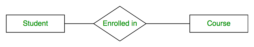
A set of relationships of the same type is known as a relationship set. The following relationship set depicts S1 as enrolled in C2, S2 as enrolled in C1, and S3 as registered in C3.

📌 Definition

The degree of a relationship is the number of entity sets participating in that relationship.

1️⃣ Unary Relationship (Degree = 1)

Only one entity is involved
Also called recursive relationship

Example:

Employee manages Employee
👉 One entity related to itself

2️⃣ Binary Relationship (Degree = 2)

Two entities are involved (most common)

Example:

Customer places Order

3️⃣ Ternary Relationship (Degree = 3)

Three entities are involved

Example:

Supplier supplies Product to Store

4️⃣ N-ary Relationship (Degree = n)

More than 3 entities

=====================================================================

✅ ACID Properties in Databases

ACID properties are fundamental principles that ensure reliability, consistency, and integrity in database transactions.

Every relational database, including Teradata, adheres to these principles for transaction management.

🔹 What is a Transaction?

A transaction is a unit of work performed in a database. It can consist of one or more SQL statements (INSERT, UPDATE, DELETE).

It ensures data integrity, especially in concurrent and failure-prone environments.

🧾 Example: Transferring ₹100 from Account A to B:

Check balance
Deduct from A
Add to B
All must succeed, or none should apply.

🔹 ACID Properties

Property	Description	Example
A – Atomicity	“All or nothing” – a transaction either completes fully or rolls back	If a money transfer fails after debiting account A but before crediting B, the debit is undone
C – Consistency	Ensures database rules and constraints are always met Database remains in a valid state before and after	If a table requires `salary > 0`, an update setting `salary = -100` is rejected
I – Isolation	Concurrent transactions do not interfere; results appear as if transactions executed serially	Two users updating the same row: isolation ensures correct final value
D – Durability	Once a transaction is committed, changes are permanent, even after a crash	After committing a purchase, the order remains recorded in the database

🔹 ACID in Teradata

Teradata supports ACID transactions at the statement level and multi-statement level
Fallback and journaling help maintain durability and fault tolerance
LOCKING mechanisms maintain isolation

🔹 Why ACID is Important

Ensures data integrity
Prevents data corruption during failures
Supports concurrent access safely
Critical for financial, healthcare, and critical systems

📈 Advantages of ACID

Ensures Data Consistency and Integrity
Concurrency control via isolation
Enables Recovery after failures

⚠️ Disadvantages

Performance overhead
Complexity in distributed systems
May limit scalability under heavy load

🌍 Where ACID is Critical

Banking: Funds transfer, balance updates
E-commerce: Inventory and order consistency
Healthcare: Patient record accuracy
Enterprise ERP/CRM: Complex transactional workflows

=====================================================================

What is Data Quality?

Data Quality (DQ) refers to the accuracy, completeness, consistency, and reliability of data in a database or data warehouse.

High-quality data ensures trustworthy analytics, reporting, and decision-making.

Poor data quality can lead to wrong business decisions, inefficiencies, and increased costs.

In simple terms:
👉 “Is your data good enough to trust and use for decisions?”

ACCT UVI

🔹 Common Data Quality Issues

Duplicate records – Same customer entered multiple times
Missing values – Important columns are NULL or empty
Incorrect data – Wrong numeric values, typos in text fields
Inconsistent formats – Dates in multiple formats (DD/MM/YYYY vs MM-DD-YYYY)
Orphan records – Foreign key refers to a non-existent primary key
Data drift – Data becomes outdated over time

🔹 Example – Checking Missing Values


SELECT emp_id, name
FROM employee
WHERE phone IS NULL;

🔹 Example – Removing Duplicate Records


DELETE FROM employee
WHERE emp_id NOT IN (
    SELECT MIN(emp_id)
    FROM employee
    GROUP BY name, phone
);

Keeps only one record per unique combination of name and phone

=====================================================================

✅ Subquery in SQL

A subquery (also called an inner query or nested query) is a query inside another SQL query. It is used to return data that will be used by the main (outer) query.

Subqueries help break down complex problems, filter data dynamically, and perform calculations or lookups within a query.

🔹 Types of Subqueries

1️⃣ Non-Correlated Subquery


SELECT emp_id, name
FROM employee
WHERE dept_id = (SELECT dept_id 
                 FROM department 
                 WHERE dept_name = 'Finance');

Inner query runs once
Returns a value for outer query to filter

2️⃣ Correlated Subquery


SELECT e1.emp_id, e1.name, e1.salary
FROM employee e1
WHERE e1.salary > (SELECT AVG(e2.salary)
                   FROM employee e2
                   WHERE e1.dept_id = e2.dept_id);

Inner query depends on each row of outer query
Calculates average salary per department dynamically

3️⃣ Subquery in SELECT


SELECT emp_id, name,
       (SELECT dept_name 
        FROM department 
        WHERE department.dept_id = employee.dept_id) AS dept_name
FROM employee;

Returns department name inline for each employee

4️⃣ Subquery in FROM (Derived Table)


SELECT dept_id, AVG(salary) AS avg_salary
FROM (SELECT dept_id, salary FROM employee) AS emp_sub
GROUP BY dept_id;

Treats subquery as a temporary table

🔹 Advantages of Subqueries

✔ Makes queries modular and readable
✔ Can replace joins in some scenarios
✔ Useful for dynamic filtering and calculations
✔ Supports nested aggregations

=====================================================================

Data Warehouse

A Data Warehouse (DW) is a centralized REPOSITORY used to store large volumes of historical, structured data from multiple sources for reporting and analytics.

👉 It is mainly used for business intelligence (BI) and decision-making.
👉 It is optimized for OLAP (Online Analytical Processing).

🔹 Popular Data Warehouse Platforms

Teradata
Amazon Redshift
Snowflake
Google BigQuery
Azure Synapse Analytics

=====================================================================

Data Mart

A Data Mart is a subset of a Data Warehouse designed for a specific department or business function (like Sales, Finance, HR).

👉 It contains focused, subject-specific data.
👉 Used for faster reporting for a particular team.

🔹 Example

If a company has a Data Warehouse containing all data:

Sales team needs only sales data
Finance team needs only revenue & expense data

👉 Separate Data Marts are created for each team.

🔹 Types of Data Mart

📌 1️⃣ Dependent Data Mart

📌 2️⃣ Independent Data Mart

📌 3️⃣ Hybrid Data Mart

👉 Balanced approach

🔹 Quick Comparison Table

Feature	Dependent	Independent	Hybrid
Source	Data Warehouse	Operational systems	Both
Data Consistency	High	Medium	High
Implementation Speed	Medium	Fast	Medium
Best For	Large organizations	Small teams	Mixed requirements

=====================================================================

What is a Database?

A database is an organized collection of data stored electronically so it can be easily accessed, managed, and updated.

🔹 1. Relational Database (RDBMS)

A Relational Database stores data in tables (rows & columns) and follows the relational model (introduced by Edgar F. Codd in 1970).

✔ Table-based
✔ Uses SQL
✔ Strong consistency
✔ Good for structured data

Example: Teradata, Oracle

🔹 2. NoSQL Database

A NoSQL database (often standing for "Not Only SQL") is a type of database designed to store and manage data that doesn't fit neatly into the traditional rows-and-columns format of standard relational databases.

✔ Non-relational
✔ Flexible schema
✔ Used for big data & real-time apps

Types of NoSQL:

Type	Example
Document	MongoDB
Key-Value	Redis
Column-family	Apache Cassandra
Graph	Neo4j

🔹 3. Hierarchical Database

Data stored in tree structure (Parent → Child)
Example: IBM Information Management System

🔹 4. Network Database

Many-to-many relationships
More flexible than hierarchical

🔹 5. Object-Oriented Database

Stores data as objects (like OOP concepts)
Supports classes, inheritance

🔹 6. Distributed Database

Data stored across multiple locations
Used in large enterprise systems

=====================================================================

✅ What is a Data Model?

A Data Model is the structured design of how data is stored, organized, and related inside a database or data warehouse.

👉 Simple meaning:
Blueprint of database structure

✅ Types of Data Models (High Level)

There are 3 levels of data modeling:

Type	Purpose	Used By
1️⃣ Conceptual	High-level business view	Business stakeholders
2️⃣ Logical	Detailed structure without DB specifics	Data architects
3️⃣ Physical	Actual implementation in DB	Developers / DBAs

1️⃣ Conceptual Data Model

A Conceptual Data Model (CDM) is the highest-level representation of data in a system.

It focuses on:

Business entities
Relationships between entities
Business rules

❌ No columns
❌ No data types
❌ No primary/foreign keys
❌ No technical details

📌 What Does It Contain?

Only 3 things:

1️⃣ Entities (High-level objects)
2️⃣ Relationships
3️⃣ High-level business rules

🧠 Example – Banking System

Conceptual view:

Customer
Account
Transaction
Branch

Relationships:

Customer owns Account
Account has Transactions
Account belongs to Branch

That’s it.

No columns like:

customer_id
account_number
transaction_date

Those come later in logical model.

Customer ---- owns ---- Account

Account ---- has ---- Transaction

Branch ---- manages ---- Account

2️⃣ Logical Data Model

A Logical Data Model defines:

Entities
Attributes (columns)
Primary Keys
Foreign Keys
Relationships
Normalization rules
Detailed structure
Entities, attributes, primary keys
No DB-specific datatype

BUT ❌ it does NOT include:

DB-specific datatypes (VARCHAR(50), INT, etc.)
Index type (PI, NUPI in Teradata)
Partitioning
Storage details

👉 It answers:
“How is the data structured logically?”

🧠 Example – Loan Origination Domain (Relevant to You)

>>Conceptual View

Since you worked on loan origination Data Vault:

Conceptual entities could be:

Customer
Loan
Channel
Application
Payment

Relationships:

Customer applies for Loan
Loan submitted via Channel
Loan has Payments

At this stage, we do NOT decide:

Hub or Satellite
Fact or Dimension
Data types
Surrogate keys

That comes in logical/physical phase.

Customer → applies → Loan
Loan → submitted via → Channel

>>Logical Data Model

Customer

Customer_ID (PK)
Customer_Name
Date_of_Birth
PAN_Number

Loan

Loan_ID (PK)
Customer_ID (FK)
Channel_ID (FK)
Loan_Amount
Loan_Status

Channel

Channel_ID (PK)
Channel_Name
Channel_Type

Notice:

✔ We added attributes
✔ Defined PK and FK
✔ Defined relationships
❌ No VARCHAR(50)
❌ No Primary Index (Teradata)

🔄 Relationship Example

1 Customer → Many Loans

So:

Customer (1)
Loan (Many)

Customer_ID becomes FK in Loan.

🔎 Normalization Happens Here

Logical modeling usually applies:

1NF – No repeating groups
2NF – Remove partial dependency
3NF – Remove transitive dependency

This is why logical models are usually highly normalized.

3️⃣ Physical Data Model

A Physical Data Model defines how data is actually implemented inside a specific database system.

It includes:

Tables
Columns
Data types
Primary key / Foreign key constraints
Indexes
Partitioning
Storage details
Performance optimization

👉 It answers:
“How will this run efficiently in a specific database?”

Actual DB implementation
Includes:

Datatypes
Indexes
Partitioning
Constraints
Storage details

🧠 Example – Loan Origination (Teradata Example)

>>Logical Model

Loan

Loan_ID
Customer_ID
Loan_Amount
Loan_Status

>>Physical Model (Teradata)


CREATE MULTISET TABLE Loan (
   Loan_ID BIGINT NOT NULL,
   Customer_ID BIGINT NOT NULL,
   Loan_Amount DECIMAL(18,2),
   Loan_Status VARCHAR(20),
   Load_Timestamp TIMESTAMP(6)
)
PRIMARY INDEX (Loan_ID);

Now we added:

✔ BIGINT
✔ DECIMAL(18,2)
✔ VARCHAR(20)
✔ PRIMARY INDEX
✔ DB syntax

That is physical modeling.


Feature Conceptual Data Model Logical Data Model Physical Data Model
🎯 Purpose Understand business requirements Define structured data design Implement in database
❓ Answers “What data is needed?” “How is data structured?” “How will it run efficiently?”
📊 Level Very High Level Medium Level Low Level (Detailed)
👥 Audience Business stakeholders, Product owners Data architects, Engineers DBAs, Engineers
📦 Entities ✅ Yes ✅ Yes ✅ Yes (as tables)
🔗 Relationships ✅ Yes ✅ Yes ✅ Yes (FK constraints)
🧾 Attributes (Columns) ❌ No ✅ Yes ✅ Yes
🔑 Primary Key ❌ No ✅ Yes ✅ Yes
🔗 Foreign Key ❌ No ✅ Yes ✅ Yes
📏 Data Types ❌ No ❌ No ✅ Yes
⚙️ Indexes ❌ No ❌ No ✅ Yes
📂 Partitioning ❌ No ❌ No ✅ Yes
🧠 Normalization ❌ No ✅ Yes Optional (may denormalize for performance)
💾 Storage Details ❌ No ❌ No ✅ Yes
🏗 DB-Specific ❌ No ❌ No ✅ Yes
🛠 Used In Requirement gathering System design Implementation & tuning
=====================================================================

Feature	Conceptual Data Model	Logical Data Model	Physical Data Model
🎯 Purpose	Understand business requirements	Define structured data design	Implement in database
❓ Answers	“What data is needed?”	“How is data structured?”	“How will it run efficiently?”
📊 Level	Very High Level	Medium Level	Low Level (Detailed)
👥 Audience	Business stakeholders, Product owners	Data architects, Engineers	DBAs, Engineers
📦 Entities	✅ Yes	✅ Yes	✅ Yes (as tables)
🔗 Relationships	✅ Yes	✅ Yes	✅ Yes (FK constraints)
🧾 Attributes (Columns)	❌ No	✅ Yes	✅ Yes
🔑 Primary Key	❌ No	✅ Yes	✅ Yes
🔗 Foreign Key	❌ No	✅ Yes	✅ Yes
📏 Data Types	❌ No	❌ No	✅ Yes
⚙️ Indexes	❌ No	❌ No	✅ Yes
📂 Partitioning	❌ No	❌ No	✅ Yes
🧠 Normalization	❌ No	✅ Yes	Optional (may denormalize for performance)
💾 Storage Details	❌ No	❌ No	✅ Yes
🏗 DB-Specific	❌ No	❌ No	✅ Yes
🛠 Used In	Requirement gathering	System design	Implementation & tuning

✅ What is SCD?

Slowly Changing Dimension (SCD) methods used to manage and track changes in dimension data over time.

🔹 SCD Type 0 – No Change

Explanation: An updated data row comes in, but we ignore that and don’t change anything.

Reasoning: We have dimensions that we don’t expect to ever change, so this new data is likely a duplicate, or just faulty data.

Example: If we assume the user inputs it correctly the first time, we never expect their date of birth to change. Unless you’re faking a birth certificate, it’s not plausible.

Ignore changes
Keep original value forever

Rarely used.

🔹 SCD Type 1 – Overwrite

Explanation: An updated data row comes in, then we overwrite the existing row completely.

Reasoning: We have dimensions that only care about the current state, so we remove any outdated rows in favour of updated rows.

Example: Nicholas Cage and Jake Peralta have updated their data. They changed their mobile phone numbers.

✔ No history
✔ Update existing record

Old value lost ❌

Use Case:

Correction of spelling mistake
Non-historical data

🔹 SCD Type 2 – Maintain Full History ⭐ (Most Important)

Explanation: An updated data row comes in, so we append a new row to the table. We don’t remove any data. To help distinguish between the two, we have up to 3 new columns:

A start date column - when this entry was processed by our data pipeline

An end date column - when this entry ended (if it hasn’t ended, you can opt for 31–12–9999, to indicate that it will never end in our lifetime)

A version number column - 1 indicates the first version, then increments upwards by 1 with every update

✔ Keep old record
✔ Insert new record
✔ Use surrogate key
✔ Track start & end dates

Reasoning: We have dimensions that we want to update, but we don’t want to lose historical data in the process.

🔹 SCD Type 3 – Limited History

Explanation: An updated data row comes in, then we use a new column to keep track. Instead of just one column for the dimension, we split it into 2 - a ‘current’ column and a ‘previous’ column:

✔ Add new column
✔ Store previous value

Similar to SCD-2, we don’t remove any data.

Reasoning: We have dimensions that we want to update, but we don’t want to lose historical data in the process.

Only 1 level history.

🔹 SCD Type 4 – History Table

Explanation: Instead of keeping all the changed data in one dimension table, we create an extra ‘mini-dimension’ history table.

That way, when an updated data row comes in, we do two things:

Overwrite the current table (similar to SCD-1)

Update the historical table to keep track of the previous values (similar to SCD-2)

Current table stores latest
Separate history table stores changes

Less common.

What does this ‘history table’ contain?

A primary key column - to allow you to join back to the current table (omitted in the below diagram for simplicity)
The other columns from your dimension table - since you’re capturing the historical values of those columns (e.g. post_code)
A start date column - when this entry was processed by our data pipeline
An end date column (optional) - when this entry ended (if it hasn’t ended, you can opt for 31–12–9999, to indicate that it will never end in our lifetime)
A version number column (optional) - 1 indicates the first version, then increments upwards by 1 with every update

Reasoning: We have dimensions that we want to update, but we don’t want to lose historical data in the process. We also want to maintain a snapshot of all the current data.

Example: Nicholas Cage and Jake Peralta have once again updated their addresses:

As mentioned in the Explanation, we update the current and historical tables accordingly:

How SCD-4 handles updates (current table). Source: Author

How SCD-4 handles updates (historical table). Source: Author

🔹 SCD Type 6 – Hybrid SCD (1 + 2 + 3)

It combines:

✅ Type 1 (Overwrite)
✅ Type 2 (New row with history)
✅ Type 3 (Previous value column)

That’s why it’s sometimes called:

👉 Type 1 + Type 2 + Type 3

✔ Keep history rows (Type 2)
✔ Also keep current flag
✔ Also keep previous value column

Used in advanced DW.

Instead of choosing one, Type 6 supports all.

=====================================================================

Relational Database Terminology

🔷 1. Tables

Core structure for storing data.
Consist of rows (records) and columns (fields).
Supports indexing, primary keys, foreign keys, etc.

Columns - A column always contains the same kind of information or contains similar data.

Row - A row is one instance of all the columns in the table.

Database - The database is a collection of logically related data. Many users access them for different purposes.

Primary Key - The primary key is used to identify a row in a table uniquely. No duplicate values are allowed in a primary key column, and they cannot accept NULL values. It is a mandatory field in a table.

Foreign Key - Foreign keys are used to build a relationship between the tables. A foreign key in a child table is defined as the primary key in the parent table.

A table can have more than one foreign key. It can accept duplicate values and also null values. Foreign keys are optional in a table.

🔷 2. Views

Virtual tables based on one or more tables or views.
Do not store data physically—just SQL definitions.
Use cases:
- Restrict access to certain columns/rows.
- Simplify complex joins/queries.
- Standardize reporting logic.
It does not store data; the data comes from underlying base tables.
Can reference single or multiple tables (joins allowed).

Useful for row/column restriction, pre-joined queries, and security.

1️⃣ Creating a View


CREATE VIEW Employee_View AS
SELECT Emp_Id,
       First_Name,
       Last_Name,
       Department_No,
       BirthDate
FROM Employee;

2️⃣ Using a View

Query it like a table:


SELECT Emp_Id,
       First_Name,
       Last_Name,
       Department_No,
       BirthDate
FROM Employee_View;

Joins, WHERE, GROUP BY, aggregates can be applied on views just like tables.

3️⃣ Modifying a View

Use REPLACE VIEW to redefine an existing view.


REPLACE VIEW Employee_View AS
SELECT Emp_Id,
       First_Name,
       Last_Name,
       BirthDate,
       JoinedDate,
       Department_No
FROM Employee;

4️⃣ Dropping a View


DROP VIEW Employee_View;

5️⃣ Advantages of Views

Security: Restrict access to certain rows/columns.
Simplification: Pre-join tables for easier querying.
Bandwidth efficiency: Only required columns are fetched.
Logical abstraction: Decouples users from underlying table structure.

🔷 3. Macros

A Macro is a stored set of SQL statements that can be executed with a single command.
Can accept parameters.
Useful for repeating business logic or securing access.
Definition is stored in the Data Dictionary, but results are generated dynamically.

Example:


CREATE MACRO GetEmployee (emp_id INT)
AS (
   SELECT * FROM Employees WHERE EmployeeID = :emp_id;
);

1️⃣ Creating a Macro


CREATE MACRO Get_Emp AS
(
   SELECT Emp_Id, First_Name, Last_Name
   FROM Employee
   ORDER BY Emp_Id;
);

Macro name must be unique in the database/user.
Can contain multiple SQL statements.

2️⃣ Executing a Macro


EXEC Get_Emp;

3️⃣ Parameterized Macros

Parameters allow dynamic filtering or passing values into the Macro.
Use : to reference the parameter inside the Macro.

Syntax:


CREATE MACRO Get_Emp_Salary(Emp_Id INTEGER) AS
(
   SELECT Emp_Id, NetPay
   FROM Salary
   WHERE Emp_Id = :Emp_Id;
);

Execute Parameterized Macro:


EXEC Get_Emp_Salary(202001);

4️⃣ Replacing a Macro

Use REPLACE MACRO to redefine an existing Macro.
Privileges depend on whether the Macro exists:
- Already exists → need DROP MACRO privilege.
- Doesn’t exist → need CREATE MACRO privilege.


REPLACE MACRO Get_Emp AS
(
   SELECT Emp_Id, First_Name, Last_Name, Department_No
   FROM Employee
   ORDER BY Emp_Id;
);

5️⃣ Key Points / Advantages

Simplifies repeated SQL tasks.
Macros execute in a single transaction, ensuring consistency.
Parameterized Macros allow dynamic queries.
Only EXEC privilege is required for users.
Can include nested Macro execution via EXEC statements.

🔷 4. Triggers

A set of SQL statements that automatically executes in response to data changes (INSERT, UPDATE, DELETE).
Attached to a table.
Used for enforcing rules or auditing changes.
The trigger logic is stored in the Data Dictionary and executed automatically.
Users don’t need to explicitly call a trigger—it runs when the event occurs.

1️⃣ Types of Triggers in Teradata

Triggers in Teradata can be categorized based on timing and event:

Type	Description
BEFORE Trigger	Executes before the triggering action (INSERT, UPDATE, DELETE).
AFTER Trigger	Executes after the triggering action is completed.
INSERT Trigger	Fires when a new row is inserted into the table.
UPDATE Trigger	Fires when a column in a row is updated.
DELETE Trigger	Fires when a row is deleted from the table.

Note: Teradata primarily supports AFTER triggers; BEFORE triggers are limited.

2️⃣ Trigger Events

A trigger can be defined for one or more of the following events:

INSERT – when new records are added.
UPDATE – when existing records are modified.
DELETE – when records are removed.

3️⃣ Trigger Syntax in Teradata

Components:

REFERENCING OLD AS / NEW AS: Allows access to old or new values of the row.
FOR EACH ROW: Executes trigger once per affected row.
FOR EACH STATEMENT: Executes trigger once per SQL statement, regardless of how many rows are affected.

4️⃣ Example 1: AFTER INSERT Trigger

Assume we have a table Employee:

Emp_Id	Name	Department	Salary
101	Mike	Sales	40000
102	Robert	IT	50000

Create an audit table:


CREATE TABLE Employee_Audit
(
   Emp_Id INTEGER,
   Action_Type VARCHAR(10),
   Action_Date TIMESTAMP
);

Trigger to log inserts:


CREATE TRIGGER Employee_Insert_Audit
AFTER INSERT ON Employee
REFERENCING NEW AS new_row
FOR EACH ROW
BEGIN
   INSERT INTO Employee_Audit (Emp_Id, Action_Type, Action_Date)
   VALUES (new_row.Emp_Id, 'INSERT', CURRENT_TIMESTAMP);
END;

Every time a new employee is inserted, a record is automatically logged in Employee_Audit.

5️⃣ Example 2: AFTER UPDATE Trigger

Trigger to log salary updates:


CREATE TRIGGER Employee_Salary_Update
AFTER UPDATE OF Salary ON Employee
REFERENCING OLD AS old_row NEW AS new_row
FOR EACH ROW
BEGIN
   INSERT INTO Employee_Audit (Emp_Id, Action_Type, Action_Date)
   VALUES (new_row.Emp_Id, 'UPDATE SALARY', CURRENT_TIMESTAMP);
END;

Tracks salary changes for every employee.

6️⃣ Example 3: DELETE Trigger

Trigger to archive deleted records:


CREATE TRIGGER Employee_Delete_Archive
AFTER DELETE ON Employee
REFERENCING OLD AS old_row
FOR EACH ROW
BEGIN
   INSERT INTO Employee_Archive (Emp_Id, Name, Department, Salary, Deleted_Date)
   VALUES (old_row.Emp_Id, old_row.Name, old_row.Department, old_row.Salary, CURRENT_TIMESTAMP);
END;

Automatically moves deleted rows to an archive table.

🔷 5. Stored Procedures

A program written in SQL and stored on the database.
Can contain control-of-flow logic (IF, LOOP, etc.).
Can be scheduled, parameterized, or reused.
Example use case: ETL workflows, validations, auditing.
Supports error handling and transaction control.
Unlike macros, SPs can include conditional logic, loops, and multiple SQL statements with error handling.
SPs execute as a single unit and can return multiple result sets.

1️⃣ Advantages of Stored Procedures

Code reusability: Write once, call many times.
Encapsulation: Hides business logic from end users.
Performance: Precompiled SQL reduces parsing time.
Can implement complex logic like conditional updates, loops, exception handling.
Can reduce network traffic, as multiple SQL statements are executed in the database server.

2️⃣ Components:

IN – Input parameter (passed to procedure).
OUT – Output parameter (returned from procedure).
INOUT – Can be passed in and returned after modification.
BEGIN … END – Defines the body of the procedure.
Supports SQL statements (SELECT, INSERT, UPDATE, DELETE) and control flow statements (IF, CASE, WHILE, FOR, LOOP).

3️⃣ Example 1: Simple Stored Procedure

Goal: Retrieve employee salary by Employee ID.


CREATE PROCEDURE Get_Emp_Salary(IN EmpId INTEGER, OUT EmpSalary INTEGER)
BEGIN
   SELECT NetPay 
   INTO :EmpSalary
   FROM Salary
   WHERE Emp_Id = :EmpId;
END;

Execution:


CALL Get_Emp_Salary(202001, ?);

? is used to capture the output parameter.
Returns the NetPay of employee 202001.

4️⃣ Example 2: Stored Procedure with Conditional Logic

Goal: Give a bonus to employees based on salary.


CREATE PROCEDURE Give_Bonus(IN EmpId INTEGER)
BEGIN
   DECLARE CurrentSalary INTEGER;

   -- Retrieve current salary
   SELECT NetPay INTO :CurrentSalary
   FROM Salary
   WHERE Emp_Id = :EmpId;

   -- Conditional logic
   IF CurrentSalary < 50000 THEN
      UPDATE Salary
      SET NetPay = NetPay + 5000
      WHERE Emp_Id = :EmpId;
   ELSE
      UPDATE Salary
      SET NetPay = NetPay + 2000
      WHERE Emp_Id = :EmpId;
   END IF;
END;

Execution:


CALL Give_Bonus(202001);

Adds a bonus dynamically based on salary.

5️⃣ Example 3: Stored Procedure with Loop

Goal: Increase salary of all employees in a department by 10%.


CREATE PROCEDURE Increase_Department_Salary(IN DeptNo INTEGER)
BEGIN
   DECLARE EmpId INTEGER;
   DECLARE done INTEGER DEFAULT 0;
   DECLARE cur1 CURSOR FOR 
       SELECT Emp_Id FROM Employee WHERE Department_No = :DeptNo;
   DECLARE CONTINUE HANDLER FOR NOT FOUND SET done = 1;

   OPEN cur1;
   loop1: LOOP
      FETCH cur1 INTO :EmpId;
      IF done = 1 THEN 
         LEAVE loop1; 
      END IF;
      UPDATE Salary
      SET NetPay = NetPay * 1.10
      WHERE Emp_Id = :EmpId;
   END LOOP loop1;
   CLOSE cur1;
END;

Execution:


CALL Increase_Department_Salary(1);

Loops through all employees in Department 1 and increases their salary by 10%.

6️⃣ Drop a Stored Procedure


DROP PROCEDURE <procedure_name>;
Key Differences
Feature Macro Stored Procedure
🎯 Purpose Execute a set of SQL statements Perform complex logic with control flow
🧠 Logic Support ❌ No procedural logic ✅ Supports IF, LOOP, WHILE
🔁 Reusability ✅ Yes ✅ Yes
⚙️ Execution Precompiled SQL Compiled procedural program
📥 Parameters ❌ Not supported ✅ Supported
📤 Return Values ❌ No ✅ Yes (via OUT params / result sets)
🔄 Control Flow ❌ No branching or loops ✅ Full control flow
⚡ Performance Faster (simple execution) Slightly slower (due to logic handling)
🛠 Complexity Simple Complex
📦 Use Case Reusable SQL queries Business logic, validations, ETL

Feature	Macro	Stored Procedure
🎯 Purpose	Execute a set of SQL statements	Perform complex logic with control flow
🧠 Logic Support	❌ No procedural logic	✅ Supports IF, LOOP, WHILE
🔁 Reusability	✅ Yes	✅ Yes
⚙️ Execution	Precompiled SQL	Compiled procedural program
📥 Parameters	❌ Not supported	✅ Supported
📤 Return Values	❌ No	✅ Yes (via OUT params / result sets)
🔄 Control Flow	❌ No branching or loops	✅ Full control flow
⚡ Performance	Faster (simple execution)	Slightly slower (due to logic handling)
🛠 Complexity	Simple	Complex
📦 Use Case	Reusable SQL queries	Business logic, validations, ETL

🔷 6. Indexes

Used to optimize data access.
Types:

Primary Index (UPI/NUPI) – determines data distribution.
Secondary Index – improves access for non-primary keys.
Join Index – speeds up joins.
Hash Index – supports fast lookups (less common now).

⚠️ Impact of Index on Writes

❌ Slows down writes

Why?

Every write = extra work
Insert row + update index
Update row → update index
Delete row → remove from index

🧾 Example

Table without index:

Insert → just add row ✅ (fast)

Table with index:

Insert → add row + update index ❌ (slower)

=====================================================================

🔥 Materialized View (MV)

A materialized view is a physical copy of a query result that is stored on disk and refreshed periodically or on demand.

👉 Unlike a normal view (which runs the query every time), a Materialized View stores precomputed results.

🔥 How It Works

When you create a Materialized View:

Query is executed
Result is stored physically
Future queries read from stored result
Data must be refreshed when base table changes

🔹 Example (Generic SQL)


CREATE MATERIALIZED VIEW mv_sales_summary AS
SELECT customer_id, SUM(amount) total_sales
FROM sales
GROUP BY customer_id;

Now:


SELECT * FROM mv_sales_summary;

👉 No aggregation runs again — data is already stored.

🔥 Refresh Types

1️⃣ Manual Refresh


REFRESH MATERIALIZED VIEW mv_sales_summary;

2️⃣ Automatic Refresh

ON COMMIT
Scheduled refresh

🔥 Advantages

✅ Faster reporting
✅ Reduces heavy joins
✅ Saves CPU
✅ Good for data warehouse

🔥 Disadvantages

❌ Uses storage
❌ Needs refresh management
❌ Slower DML on base tables

🔥 Materialized View in Teradata

In Teradata Vantage, there is no direct "Materialized View" keyword.

👉 Instead, Teradata uses:

Join Index
Summary Tables
Aggregate Join Index

These work like materialized views.

Example (Teradata style using Join Index):


CREATE JOIN INDEX mv_sales_summary AS
SELECT customer_id, SUM(amount) total_sales
FROM sales
GROUP BY customer_id
PRIMARY INDEX (customer_id);

🔥 When to Use Materialized View?

✔ Heavy aggregation queries
✔ Repeated reporting queries
✔ Large joins
✔ Data warehouse systems

=====================================================================

Teradata Components

Teradata Corporation built Teradata using MPP (Massively Parallel Processing) architecture.

🔹 1️⃣ Parsing Engine (PE)
The Parsing Engine is a virtual processor (vproc) that interprets SQL requests, receives input records, and passes data.

To do that, it sends the messages over the BYNET to the AMPs (Access Module Processor).

👉 PE does NOT store data.

🔹 2️⃣ BYNET

This is the message-passing layer or simply the networking layer in Teradata.

It receives the execution plan from the parsing engine and passes it to AMPs and the nodes.

After that, it gets the processed output from the AMPs and sends it back to the parsing engine.

To maintain adequate availability, the BYNET 0 and BYNET 1 two types of BYNETs are available. This ensures that a secondary BYNET is available in case of the failure of the primary BYNET.

Feature	Explanation
High-speed network	Connects nodes
Message passing	Transfers data between AMPs
Parallel communication	Enables MPP processing

👉 Acts like backbone network.

🔹 3️⃣ AMP (Access Module Processor)

These are the virtual processors of Teradata. They receive the execution plan and the data from the parsing engine.

The data will undergo any required conversion, filtering, aggregation, sorting, etc., and will be further sent to the corresponding disks for storage.

The AMP is a virtual processor (vproc) designed for and dedicated to managing a portion of the entire database.

The AMP receives data from the PE, formats rows, and distributes them to the disk storage units it controls. The AMP also retrieves the rows requested by the Parsing Engine.

Table records will be distributed to each AMP for data storage.

Function	Explanation
Data Storage	Stores actual table data
Data Retrieval	Fetches rows
Index Handling	Manages primary index
Parallel Processing	Each AMP works independently

👉 Data is distributed across AMPs.

🔹 4️⃣ Node

The basic unit of a Teradata system is called a Node.

Each node has its operating system, CPU memory, a copy of RDBMS software, and some disk space. A single cabinet can have one or more nodes in it.

A Node is a physical server in the Teradata system.

It includes both hardware and software components that support the execution of Teradata’s parallel database processing.

Feature	Description
Physical Server	Runs Teradata software
Contains	Multiple AMPs + PE
Scalable	Add nodes to scale system

🔹 Parallel Database Extensions (PDE)

The Parallel Database Extensions is a software interface layer that lies between the operating system and database. It controls the virtual processors (vprocs).

🔹 Disks

Disks are disk drives associated with an AMP that store the data rows. On current systems, they are implemented using a disk array.

🔄 Query Execution Flow in Teradata

Query Submission
A user or application submits an SQL query.
Parsing Engine (PE)
- Parser: Checks SQL syntax and semantics.
- Security: Validates user access.
- Optimizer: Generates the most cost-effective execution plan.
- Dispatcher: Sends the execution steps to BYNET.
BYNET
Routes the steps from the PE to the appropriate AMPs.
AMPs (Access Module Processors)
- Execute the steps (e.g., read/write data).
- Retrieve or update data from their own disks.
- Send results back to the PE.
PE (again)

Assembles the rows.
Sends the final result back to the client.

=====================================================================

Index Types in Teradata

In Teradata, indexes are mainly used for data distribution and faster retrieval.

1️⃣ PI (Primary Index)

The Primary Index (PI) is the core mechanism for distributing rows across AMPs and retrieving data efficiently.

Primary Index decides:

Decides where the data is stored (which AMP).
Mandatory (every table must have one).
How data is distributed

👉 Every table MUST have one PI
👉 It does NOT have to be unique

✅ Key Characteristics

Attribute	Description
Purpose	Determines how rows are distributed and accessed
When defined?	At CREATE TABLE time only – cannot be altered later
Max Columns	Can consist of 1 to 64 columns
Stored in	Data Dictionary (DD)

🧠 Best Practices for Choosing a PI

Choose a highly unique column to avoid skew (UPI preferred).
Consider query access patterns (frequent filters, joins).
Try to align PI with foreign keys in child tables for AMP-local joins.
Avoid columns with few distinct values (e.g., Gender, Status) as PI → causes skew.

📈 Why PI Matters for Performance

Every row access by PI is a 1-AMP operation → fastest.
Good PI choice = even AMP workload → maximum parallelism.
Bad PI choice = skew → one AMP overworked, others underutilized.

🚫 Common Mistakes

Using low cardinality columns as PI (e.g., "India", "Yes/No").
Forgetting that PI ≠ PK in Teradata.
Choosing PI without analyzing access patterns.

🔹 2️⃣ UPI (Unique Primary Index)

A Primary Index where column values are unique.

👉 No duplicate values allowed
👉 Best performance
👉 Even data distribution

🔹 3️⃣ NUPI (Non-Unique Primary Index)

Primary Index where duplicates are allowed.

The hashing algorithm still determines the target AMP, but:

All rows with the same NUPI value go to the same AMP.
This can lead to uneven (skewed) distribution.

Example: Skew from Poor NUPI Choice
If you choose Order_Status (values = "C", "O") as a NUPI:

All rows get hashed to just 2 AMPs.
Remaining AMPs stay idle → severe performance degradation.

👉 Most commonly used
👉 Can cause data skew if not chosen properly

If many rows have same cust_id → skew risk.

🔹 4️⃣ SI (Secondary Index)

A Secondary Index (SI) is an additional index created on a column other than the Primary Index to improve query performance.

A Secondary Index (SI) in Teradata is a physical access path to the data that is separate from the Primary Index (PI).

It is used to improve query performance when the query's search condition does not use the PI columns.

👉 It does NOT control data distribution
👉 It helps in faster data retrieval
👉 It uses extra storage

🔍 Why Use a Secondary Index?

When queries frequently use non-PI columns in WHERE conditions.
To avoid full table scans.
To reduce query response time.
To optimize joins or aggregations on non-PI columns.

Additional index created for faster search on non-PI columns.

Optional
Improves query performance
Requires extra storage
SI is optional
Used for non-PI columns
Improves read performance
Increases write overhead

🚦 Performance Tips

USI: Great for point queries (e.g., WHERE emp_name = 'Alice')
NUSI: Better for range queries (e.g., WHERE salary BETWEEN 50000 AND 70000)
Too many SIs can increase storage and slow down DML operations like INSERT/UPDATE.

🔹 5️⃣ USI (Unique Secondary Index)

A Unique Secondary Index (USI) is a secondary index created on a column where duplicate values are NOT allowed.

👉 Ensures uniqueness
👉 Used for fast lookup
👉 Stored in a separate index subtable

👉 Secondary index with unique values
👉 Stored in separate subtable
👉 Very fast lookup

🔹 How USI Works Internally

User runs query:


SELECT * FROM customer WHERE email_id = 'rk@gmail.com';

Teradata hashes the USI column
Goes to specific AMP storing USI subtable
Finds RowID
Fetches actual row from base table

👉 Very fast because it’s unique.

🔹 6️⃣ NUSI (Non-Unique Secondary Index)

A Non-Unique Secondary Index (NUSI) is a secondary index created on a column where duplicate values are allowed.

👉 Used for filtering
👉 Improves SELECT performance
👉 Does NOT control data distribution

👉 Allows duplicates
👉 Stored on same AMP
👉 Helps filtering

🔹 How NUSI Works Internally

Query runs:


SELECT * FROM orders WHERE status = 'SHIPPED';

Teradata checks NUSI subtable
Finds list of RowIDs for matching rows
Fetches rows from base table

👉 Since duplicates exist, multiple rows are returned.

✅ What is a NoPI Table?

A NoPI (No Primary Index) Table is a table that does not have a defined Primary Index.

This was introduced in Teradata 13.0 to improve bulk load performance and simplify certain workloads.

CREATE TABLE table_x
 	(col_x INTEGER
 	,col_y CHAR(10)
 	,col_z DATE)
NO PRIMARY INDEX;

📦 Why Use NoPI Tables?
Ideal for staging or landing tables in ETL pipelines.
Great for bulk loading large volumes of data quickly.
Often used temporarily before redistributing data into final structured tables.
🧠 Best Practices:
Use NoPI tables for staging or intermediate ETL steps.
Avoid long-term use unless you really do not need joins or indexed access.
After loading, redistribute data into base tables with a PI for performance.

=====================================================================

🚀 How Teradata Distributes Rows Across AMPs

In Teradata, row distribution is fully automatic, even, and hash-based.

The core idea is that each AMP (Access Module Processor) is responsible for a portion of each table’s data, and Teradata ensures the rows are distributed evenly using a hashing algorithm.

🔁 Hash-Based Distribution Mechanism

When a row is inserted into a table:

Teradata hashes the Primary Index column(s) value.
The resulting hash value is mapped to an AMP.
That AMP stores the row on its associated disk.

📌 Hashing is done on Primary Index (PI) — it’s how Teradata determines where to store a row.

🎯 Why Even Distribution Matters

Ensures parallelism is fully utilized.
Avoids skew (when some AMPs hold significantly more rows than others).
Prevents slowest AMP bottleneck in full table operations.

✅ Ideally:

Each table's rows are evenly distributed across all AMPs.
All AMPs perform roughly equal work on large queries.

🔄 Row Distribution Mechanism

Teradata uses a hashing algorithm on the PI column(s).
Hash result determines the AMP where the row will be stored.
Leads to parallelism across AMPs.

📥 How Data Gets Distributed Across AMPs

When a row is inserted into a Teradata table:

The Primary Index (PI) value of the row is input into a hashing algorithm.
The algorithm outputs a 32-bit Row Hash.
The high-order 16 bits are used to find a Hash Bucket Number.
The Hash Map uses that bucket number to determine which AMP will store the row.
The AMP stores the row in its associated vDisk.

Teradata Hashing Algorithm

Teradata uses a hashing algorithm to determine which AMP (Access Module Processor) stores a row.

Every row in Teradata is distributed to an AMP based on its Primary Index (PI) value.
The hashing algorithm transforms the PI into a 32-bit RowHash, which is used to identify the AMP.

1️⃣ How Hashing Works (Step-by-Step)

Client submits query → provides the Primary Index value of the row.
Parser receives the query and passes the PI value to the hashing algorithm.
Hashing algorithm generates a 32-bit RowHash from the PI value.
High-order bits of the RowHash (first 16 bits) determine the Hash Bucket.
Hash Map maps the Hash Bucket to a specific AMP.
BYNET sends the row to the identified AMP.
AMP uses the RowHash to locate the row on disk.
If multiple rows have the same RowHash, a uniqueness ID is incremented.
Combination of RowHash + Uniqueness ID → RowID, which uniquely identifies each row.
Rows on the AMP are logically stored sorted by RowID

2️⃣ Hashing Functions in Teradata

Function	Description	Syntax
HASHROW	Returns 32-bit RowHash for a column or expression.	`HASHROW(col1 [, col2 ...])`
HASHAMP	Returns the primary AMP number for a given Hash Bucket.	`HASHAMP(hashbucket)`
HASHBUCKET	Returns 16-bit Hash Bucket used with the Hash Map to locate the AMP.	`HASHBUCKET(col1 [, col2 ...])`
HASHBAKAMP	Returns the fallback AMP number for a given Hash Bucket.

MP Returns the fallback AMP number for a given Hash Bucket. HASHBAKAMP(hashbucket)

3️⃣ Example

Tables


CREATE SET TABLE Employee (
   Employee_Id INTEGER,
   Name VARCHAR(10),
   Salary INTEGER
) PRIMARY INDEX(Employee_Id);

How a row is assigned:

Employee_Id = 1001
HASHROW(1001) → 32-bit RowHash = 0xABCD1234 (example)
High-order 16 bits → Bucket number = 43981
Hash Map → AMP #2 → row stored on AMP 2
RowID = RowHash + Uniqueness ID → uniquely identifies the row.

4️⃣ Hash Collisions

Hash Collision: Two different PI values produce the same RowHash → same Hash Bucket.
Teradata avoids collisions with:
1. Uniqueness ID → incremented for rows with same RowHash.
2. RowID → 64-bit combination of RowHash + Uniqueness ID → unique row identifier.

✅ Even if multiple rows share the same Hash Bucket, Teradata can efficiently locate the correct row using RowID.

5️⃣ Hash Map

Hash map is a translation table mapping Hash Buckets → AMP numbers.
Each hash bucket in the map is assigned to a specific AMP.
BYNET uses the hash map to route data to the correct AMP.

6️⃣ Visual Overview


[Client Query] → Parser → Hashing Algorithm → RowHash (32-bit)
    → High-order bits → Hash Bucket → Hash Map → AMP
    → AMP stores row with RowID (RowHash + Uniqueness ID)

=====================================================================

Partitioned Primary Index (PPI)

PPI is a Teradata feature that divides rows into partitions based on a defined column or expression, while still distributing rows across AMPs based on the Primary Index (PI).

👉 Data is distributed across AMPs (like normal PI)
👉 Within each AMP, data is divided into partitions
👉 Improves range query performance

A Partitioned Primary Index (PPI) helps avoid full table scans by physically organizing rows in partitions based on column values.

Within each partition, rows are ordered by RowHash (used by AMP for distribution).
Queries on partitioned columns access only relevant partitions, improving performance.

Key Benefits:

Improves query performance for range-based queries.
Allows partition elimination, where irrelevant partitions are excluded at query time.
Ideal for incremental loads, archiving, and deletions.

⚙️ How PPI Works:

Hashing for Distribution:
- PI → Hash Value → Determines which AMP stores the row.
Partitioning for Storage Order:
- Once inside an AMP, rows are grouped into partitions.
- Within each partition, data is sorted by Row Hash (row ID).
Partition Elimination:

The optimizer analyzes query filters (e.g., WHERE order_date BETWEEN …) and skips partitions that won’t qualify.
This reduces I/O and scan time dramatically.

SELECT * FROM sales WHERE oder_date= DATE '2024-05-10';

👉 Only May partition scanned
👉 Faster query


SELECT *
FROM Sales
WHERE SaleDate = DATE '2024-05-10';

👉 Optimizer scans only May partition
👉 Other partitions skipped
👉 This is called Partition Elimination

You do NOT need to mention PARTITION.


SELECT *
FROM Sales
WHERE PARTITION = 5;

👉 Fetches rows only from partition 5
⚠ Not commonly used in business queries
⚠ Mostly for debugging / admin usage

🔹 Query


SELECT *
FROM Sales
WHERE PARTITION < 6;

🔎 What it means

👉 Return rows from Partition 1 to 5

So it returns data for:

🔹 When NOT to Use PPI

❌ Small tables
❌ Queries without filter on partition column
❌ Very high insert workloads (slightly more overhead)

PARTITION BY RANGE_N(

totalorders BETWEEN *, 100, 1000 AND *,

UNKNOWN

);

🌲 Multilevel Partitioned Primary Index (MLPPI)

MLPPI allows sub-partitioning — i.e., a partition within a partition — for greater granularity and performance.

Example Use Case:

Partition 1: by Claim_Date
Sub-partition: by State

This improves query efficiency when filters match both levels, enabling multi-level partition elimination.

In Teradata, when using Multi-Level Partitioned Primary Index (MLPPI), you can define the partitions using either:

RANGE_N — for range-based partitioning (like dates, numbers)
CASE_N — for custom logic or discrete values

🧩 Use `RANGE_N` When:

You are partitioning by a range of values (e.g., dates or numeric ranges).
Best for time-series data, like logs or transaction tables.

🧩 Use `CASE_N` When:

You want to partition using categorical values, custom conditions, or non-uniform ranges.
Good when data doesn't fit into neat, equal ranges.

=====================================================================

Teradata Columnar (Column Partitioning)

Column Partitioning stores columns separately instead of storing full rows together.

👉 Traditional Teradata = Row-based storage
👉 Column Partitioning = Column-based storage
👉 Improves performance for analytical queries

It can be applied to:

Tables (especially NoPI tables)
Join Indexes

🔹 Normal Table (Row Storage)

If table has 20 columns:


SELECT col1, col2 FROM big_table;

👉 Teradata reads all 20 columns from disk
👉 Higher I/O

🔹 Column Partitioning

👉 Data stored column-wise
👉 Only required columns read

SELECT col1, col2 FROM big_table;

👉 Only col1 and col2 scanned
👉 Reduced I/O
👉 Faster query

🔹 Limitations

❌ Slightly slower inserts
❌ Not ideal for transactional workloads
❌ More complex storage structure

=========================================================================

Join Index (JI) in Teradata

A Join Index is a system-maintained physical structure that stores pre-joined or pre-aggregated data

of join of two or more tables to speed up query performance.

👉 Reduces repeated join computation
👉 Stored physically like a table
👉 Can be row-based or columnar (Columnar Join Index = CJI)

Eliminate base table joins
Reduce data redistribution
Avoid aggregate processing
Improve query response time

🔷 1. What is a Single-Table Join Index (STJI)?

A Single-Table Join Index is a special type of join index that:

Is defined on only one table.
Uses a different column as its Primary Index (PI) than the base table’s PI.
Helps optimize joins between foreign keys and primary keys—especially in star schema or snowflake models.
Avoids row redistribution and base table access during queries.

🧩 Why Use STJI?

Teradata stores rows based on the PI. If you frequently join on a non-PI column (e.g., a foreign key), Teradata may redistribute data to perform the join.

✅ STJI prevents redistribution by pre-sorting and rehashing rows using the foreign key (or any chosen column).

What This Does:

Creates a copy of the orders table, hashed on customer_id instead of order_id.
When a query joins orders.customer_id to customers.customer_id, Teradata can use this index.
No data redistribution needed because both tables are now hashed on the same column.

🔹 2.Multi-Table Join Index (MTJI) in Teradata

A Multi-Table Join Index (MTJI) is a Join Index that combines more than two base tables into a precomputed, stored join.

👉 Speeds up queries that join multiple tables frequently
👉 Can be row-based or columnar
👉 Stored physically like a table

🔹 Advantages

✅ Speeds up multi-table queries
✅ Reduces CPU & AMP load
✅ Precomputed join simplifies SQL
✅ Good for data warehouse reporting

🔹 Disadvantages

❌ Uses extra disk space
❌ Slower inserts/updates/deletes on base tables (index maintenance)
❌ Needs careful design to select only necessary columns

🔹 3. Aggregate Join Index (AJI) in Teradata

An Aggregate Join Index (AJI) is a precomputed, stored table that combines aggregation and joins.

👉 Optimized for analytical queries
👉 Stores aggregated values (SUM, COUNT, AVG, etc.)
👉 Can be row-based or columnar
👉 Reduces query processing time on large fact tables

🔹 Advantages

✅ Improves query performance for aggregation queries
✅ Reduces CPU and I/O on large tables
✅ Simplifies complex queries for users
✅ Can be combined with columnar storage for further optimization

🔹 Disadvantages

❌ Extra storage required
❌ Insert/Update/Delete slower due to maintenance
❌ Needs careful selection of aggregation columns

🔹 4. Columnar Join Index (CJI) in Teradata

A Columnar Join Index (CJI) is a precomputed, columnar storage index based on a join of one or more tables to improve query performance for analytical workloads.

👉 Combines benefits of Join Index (prejoin data) and Columnar storage (column-based access)
👉 Speeds up queries with aggregations, filters, and joins

🔹 How Columnar Join Index Works

1️⃣ Base tables: sales and customer

2️⃣ Query often executed:


SELECT c.region, SUM(s.amount)
FROM sales s
JOIN customer c
ON s.cust_id = c.cust_id
GROUP BY c.region;

3️⃣ CJI created:


CREATE JOIN INDEX cji_sales_customer AS
SELECT s.amount, c.region
FROM sales s
JOIN customer c
ON s.cust_id = c.cust_id
PRIMARY INDEX (cust_id)
PARTITION BY COLUMN;

Stores only needed columns (amount and region)
Precomputed join stored in columnar format
Queries hitting CJI skip join computation

=========================================================================

🔍 Full Table Scan (FTS)

A Full Table Scan happens when Teradata (or any database engine) reads every row in a table to find rows that match a query’s condition—because no index or partitioning strategy can narrow it down.

⚠️ This is often the least efficient way to access data, especially for large tables.

❌ What happens here?

The Primary Index (PI) is on emp_id, but the query filters on dept_id, which is not indexed.
Result: Teradata must read every row to find those where dept_id = 10 → Full Table Scan.

=========================================================================

✅ Best Practices

Choose PKs based on business rules and uniqueness.
Choose PIs based on query patterns, join usage, and data distribution.
Don't always assume PK = PI. Analyze based on performance needs.

=====================================================================

🔹 Compression in Teradata

In Teradata, Compression is used to reduce storage space and improve query performance.

👉 It reduces disk usage
👉 Improves I/O performance
👉 Saves storage cost

✅ It’s especially effective in large tables with:

Repeating values (like status = ‘Active’)
Nullable columns with many nulls
Low-cardinality columns (few distinct values)

🧱 How `COMPRESS` Works

Instead of storing the full value for every row, Teradata:

Stores common/repeating values only once in the table header.
Rows with those values point to the compressed value.
Values not listed in COMPRESS are stored normally.

🔹 1️⃣ Multi Value Compression (MVC)

📌 What It Does

Stores frequently repeating values using internal codes.

Multi-value compression has three variations:

COMPRESS – ONLY Nulls are compressed.
COMPRESS NULL – Nulls are compressed. (COMPRESS & COMPRESS NULL mean the same thing)
COMPRESS <constant> – Nulls and the specified <constant> value are compressed.

📌 Example


CREATE TABLE employee (
  gender CHAR(1) COMPRESS ('M','F'),
  status VARCHAR(10) COMPRESS ('ACTIVE','INACTIVE')
);

🔹 Benefit

If 80% rows have ACTIVE, storage is reduced.

🔹 2️⃣ Block Level Compression (BLC)

Performs compression on whole data blocks at the file system level before they are written to storage.

👉 Transparent to users.

Feature	Description
Works at	Data block level
Compresses	Entire block of rows
Best For	Large tables
Enabled	Automatically in newer versions

🔹 3️⃣ Algorithmic Compression (ALC)

When column values are mostly unique, Algorithmic Compression can provide better compression results than Multi-value Compression.

You can define your own compression and decompression algorithms and apply them to data at the column level.

ALC allows you to implement the compression scheme that is most suitable for data in a particular column. The cost of compression and decompression depends on the algorithm chosen.

Feature	Description
Uses algorithm	To compress numeric patterns
Works for	Dates, integers
Storage reduction	Higher than MVC sometimes

=====================================================================

🔹 Space in Teradata

In Teradata, Space means the disk storage allocated to a database or user to store tables, indexes, temporary data, etc.

👉 Space is allocated at Database/User level
👉 Managed automatically across AMPs
👉 Measured in bytes (KB, MB, GB)

🔍 1. Perm Space

Permanent Space (Perm Space) is the disk space allocated to store permanent database objects like tables, indexes, views, macros, etc.

👉 Stores actual business data
👉 Not automatically cleared
👉 Allocated to Database/User
👉 Distributed across AMPs

Definition: Maximum allowed space a user/database can occupy permanently.
Not pre-allocated, only consumed as needed.
Used for:
- Table data (rows)
- Stored procedures
- User-Defined Functions (UDFs)
Required for creating tables.

Feature	Description
Stores	Tables, indexes, views
Allocated to	Database/User
Remains until	Object is dropped
Most important	Yes

🔍 2. Spool Space

Spool Space is temporary disk space used by Teradata to store intermediate results while executing a query.

👉 Used during SELECT, JOIN, GROUP BY, ORDER BY
👉 Automatically cleared after query finishes
👉 If exceeded → query fails

Definition: Temporary space used during SQL execution.
Used for:
- Sorting
- Joining
- Aggregation
- Storing query results
Reclaimed automatically when the query ends.
Inherits limits from parent user/database unless explicitly set.

Feature	Description
Used for	Intermediate query results
Automatically freed	After query ends
Very important	Yes (query may fail if exceeded)

🔍 3. Temp Space

Temp Space (Temporary Space) is the disk space used to store Global Temporary Tables (GTTs) during a user session.

👉 Used only for temporary tables
👉 Data is session-specific
👉 Automatically cleared after session ends

Tables created in Temp Space survive restarts (not the data).
Treated like Perm Space, but temporarily allocated for session data.

Feature	Description
Used for	Global Temporary Tables
Released	At session end
Stored in	Temp Space allocation

4️⃣ Journal Space

Journal Space is the disk space used to store before and after images of rows for data recovery purposes.

👉 Helps in recovering data if transaction fails
👉 Used for rollback and permanent journal

Feature	Description
Used for	Recovery
Stores	Before/After image of rows
Optional	Can be disabled

=====================================================================

📌 `COLLECT STATISTICS`

COLLECT STATISTICS (a.k.a. COLLECT STATS) gathers data demographics (like row count, value distribution, uniqueness) on columns, indexes, or partitions.

Collect Statistics is a process in Teradata that gathers metadata about table columns or indexes to help the optimizer choose the best execution plan.

✅ These stats are used by the Teradata Optimizer to:

Choose optimal query plans
Decide whether to use an index or full table scan
Improve join strategies, aggregations, and access paths

💡 Why It Matters

Without stats, Teradata assumes uniform distribution and guesses row counts, which can result in:

Wrong join order
Full table scans
Skewed AMP workload
Longer response times

HELP STATISTICS <tablename>;

🔹 How It Helps Optimizer

Determines row count and value distribution
Helps decide join strategy:
- Merge Join
- Hash Join
- Product Join
Helps in AMP assignment
Reduces spool space usage

📊 What Does It Collect?

Distinct values count
Null count
Min/Max values
Frequency histogram
Row count
Skew factor

These help the optimizer estimate:

Selectivity (how many rows a filter returns)
Join cardinality
Join cost and order
Whether to use an index, join index, or full table scan

🔹 SAMPLE in COLLECT STATISTICS (Teradata)

In Teradata Vantage, the SAMPLE option in COLLECT STATISTICS allows the optimizer to collect statistics using only a percentage of table rows instead of scanning the entire table.

👉 This reduces resource usage and improves performance when collecting stats on large tables.

✅ Why Use SAMPLE?

Full stats collection = Full table scan (expensive on big tables)

Using SAMPLE:

Faster
Less CPU usage
Less I/O
Less spool usage

Best for:

Very large tables
Frequently refreshed data
Columns with good distribution

🔹 Types of SAMPLE

1️⃣ SYSTEM SAMPLE (Recommended)


COLLECT STATISTICS 
USING SYSTEM SAMPLE
COLUMN (emp_id)
ON Employee;

✔ System decides optimal sample size
✔ Automatically balances accuracy vs performance

2️⃣ SAMPLE n PERCENT


COLLECT STATISTICS 
USING SAMPLE 10 PERCENT
COLUMN (emp_id)
ON Employee;

✔ You control percentage
✔ n range: 2 – 100
✔ SAMPLE 100 PERCENT = Full statistics

🔹 Full Statistics


COLLECT STATISTICS COLUMN(emp_id) ON Employee;

Scans 100% rows
More accurate
Slower

🔹 Sample Statistics (10%)


COLLECT STATISTICS 
USING SAMPLE 10 PERCENT
COLUMN(emp_id)
ON Employee;

Scans only 10% rows
Faster
Slightly less accurate

🔹 When to Use SAMPLE?

Scenario	Use SAMPLE?
Huge fact table	✅ Yes
Small table	❌ No (collect full)
Highly skewed column	❌ Better full stats
Nearly unique column	✅ Sample works well
Partitioned table	⚠ Depends

🔹 Collect Statistics on Partition Column (Teradata)

In Teradata Vantage, collecting statistics on a Partition Primary Index (PPI) column is very important for performance.

If you don’t collect stats on partition columns, the optimizer may:

Scan all partitions ❌
Misestimate row counts ❌
Generate large spool ❌

1️⃣ Basic Syntax


COLLECT STATISTICS 
COLUMN (PARTITION)
ON sales_table;

✔ COLUMN (PARTITION) is special keyword
✔ Used only for partitioned tables

2️⃣ Collect Stats on Partition + Column Together


COLLECT STATISTICS 
COLUMN (PARTITION, order_date)
ON sales_table;

✔ Helps optimizer understand:

Partition distribution
Column distribution inside partition

3️⃣ Collect Stats on Partitioned Column Normally

If table is partitioned by:


PARTITION BY RANGE_N(order_date BETWEEN DATE '2024-01-01'
AND DATE '2026-12-31'
EACH INTERVAL '1' MONTH);

You should collect:


COLLECT STATISTICS COLUMN(order_date) ON sales_table;

AND


COLLECT STATISTICS COLUMN(PARTITION) ON sales_table;

Best practice → Collect both.

🔥 Example


CREATE TABLE sales_table
(
   order_id INTEGER,
   order_date DATE,
   amount DECIMAL(10,2)
)
PRIMARY INDEX(order_id)

PARTITION BY RANGE_N(order_date 
BETWEEN DATE '2024-01-01'
AND DATE '2025-12-31'
EACH INTERVAL '1' MONTH);

Collect stats:


COLLECT STATISTICS COLUMN(PARTITION) ON sales_table;
COLLECT STATISTICS COLUMN(order_date) ON sales_table;

🔹 Why Both Needed?

Statistic	Purpose
PARTITION	Number of rows per partition
order_date	Value distribution inside partitions

Together → Better partition pruning + better join plan.

🔹 USING THRESHOLD in COLLECT STATISTICS (Teradata)

In Teradata Vantage, THRESHOLD is used in COLLECT STATISTICS to avoid unnecessary recollection of stats.

👉 It improves performance by recollecting statistics only when needed.

✅ Why THRESHOLD is Needed?

Recollecting stats every time:

Wastes CPU
Consumes I/O
Uses spool
Slows batch jobs

THRESHOLD helps skip recollection if:

Data change is small
Stats are still recent

🔹 Types of THRESHOLD

1️⃣ THRESHOLD n PERCENT (Change-Based)

Recollect only if data changed by more than n%.


COLLECT STATISTICS 
COLUMN(emp_id) 
ON employee
THRESHOLD 10 PERCENT;

👉 If data changed < 10% → stats NOT recollected
👉 If data changed ≥ 10% → stats recollected

2️⃣ THRESHOLD n DAYS (Time-Based)

Recollect only if stats older than n days.


COLLECT STATISTICS 
COLUMN(emp_id) 
ON employee
THRESHOLD 7 DAYS;

👉 If stats collected 3 days ago → skipped
👉 If stats collected 10 days ago → recollected

3️⃣ Combined THRESHOLD (Both Conditions)


COLLECT STATISTICS 
COLUMN(emp_id) 
ON employee
THRESHOLD 10 PERCENT
AND THRESHOLD 5 DAYS;

Recollection happens only if:

Change ≥ 10%
AND
Older than 5 days

🔹 Remove Threshold

NO THRESHOLD


COLLECT STATISTICS 
COLUMN(emp_id) 
ON employee
NO THRESHOLD;

Remove Only Days Threshold


NO THRESHOLD DAYS;

Remove Only Percent Threshold


NO THRESHOLD PERCENT;

🔥 First Time Collection

If stats are collected for the first time:

THRESHOLD is ignored
Stats are collected
Threshold is stored for future recollections

=====================================================================

🔹 WITH DATA Table in Teradata

In Teradata Vantage, WITH DATA is used when creating a table from another table or query, and you want to copy both:

✅ Structure (columns, datatypes)
✅ Data

🔹 Example 1 — Copy Structure + Data

Source Table


CREATE TABLE employee
(
   emp_id INTEGER,
   emp_name VARCHAR(50),
   salary DECIMAL(10,2)
);

Insert data:


INSERT INTO employee VALUES (1,'John',50000);
INSERT INTO employee VALUES (2,'Alice',60000);

Create Backup Table


CREATE TABLE employee_bkp AS employee
WITH DATA;

🔹 Example 2 — Using SELECT


CREATE TABLE high_salary_emp AS
(
   SELECT * FROM employee
   WHERE salary > 55000
) WITH DATA;


CREATE TABLE empty_emp AS employee
WITH NO DATA;

👉 Only structure copied
👉 No rows copied

🔹 WITH DATA AND STATS in Teradata

In Teradata Vantage, WITH DATA AND STATS is used to copy:

✅ Table structure
✅ Data
✅ Collected statistics

This is very useful in performance tuning scenarios.

✅ Syntax


CREATE TABLE new_table AS old_table
WITH DATA AND STATS;


CREATE TABLE new_table AS
(
   SELECT * FROM old_table
)
WITH DATA AND STATS;

🔹 What Exactly Gets Copied?

Component	Copied?
Columns	✅ Yes
Data	✅ Yes
Collected Statistics	✅ Yes
Primary Index	✅ Yes
Constraints	❌ No
Triggers	❌ No
Default values	❌ No

🔥 Why WITH DATA AND STATS is Important?

In Teradata, the optimizer depends heavily on statistics.

If you use only:


WITH DATA

The new table will have no statistics, and query performance may degrade.

But:


WITH DATA AND STATS

👉 Preserves optimizer behavior
👉 Avoids recollecting statistics
👉 Saves time in large tables

=====================================================================

MERGE USING WHEN in Teradata

MERGE INTO is used to:

👉 UPDATE existing rows
👉 INSERT new rows
👉 In a single statement

It is commonly called an UPSERT operation.

MERGE is used to synchronize two tables by performing:

Updating rows in the target table that match rows in the source table.
Inserting rows into the target table that exist in the source but not in the target
Deleting rows from the target table that do not exist in the source.

🔹 How It Works

Condition	Action
Row exists in target	UPDATE
Row does not exist	INSERT

🔥 Example

🎯 Target Table: Employee

id	name	salary
1	John	5000
2	Mike	6000

🎯 Source Table: Employee_Stage

id	name	salary
2	Mike	6500
3	Alice	7000

MERGE Query
MERGE INTO employee tgt
USING employee_stage src
ON tgt.id = src.id

WHEN MATCHED THEN
   UPDATE SET salary = src.salary

WHEN NOT MATCHED THEN
   INSERT (id, name, salary)
   VALUES (src.id, src.name, src.salary);

✅ Result After MERGE

id	name	salary
1	John	5000
2	Mike	6500
3	Alice	7000

🔹 Multiple WHEN Conditions

Teradata allows conditions inside WHEN MATCHED.


WHEN MATCHED AND tgt.salary <> src.salary THEN
   UPDATE SET salary = src.salary

👉 Update only if salary changed.

🔹 DELETE with MERGE


WHEN MATCHED AND src.status = 'D' THEN
   DELETE

Used in SCD Type 1 logic or soft delete handling.

🔥 Important Rules in Teradata

1️⃣ Target table must be a base table (not view)
2️⃣ Cannot update Primary Index column
3️⃣ Only one source row should match a target row (else error)
4️⃣ Works best when join is on PI

🔥 MERGE vs INSERT + UPDATE

Feature	MERGE	Separate INSERT + UPDATE
Single pass	✅ Yes	❌ No
Faster	✅ Yes	❌ Slower
Cleaner logic	✅ Yes	❌ More code

🔥 MERGE on Non-Equality Condition in Teradata

In Teradata Vantage, the MERGE statement is primarily designed for equality joins.

❗ Important Rule

👉 In Teradata, the ON condition of MERGE must use equality (=) conditions.

You cannot directly use:


ON tgt.date BETWEEN src.start_date AND src.end_date   ❌
ON tgt.amount > src.min_amt                           ❌
ON tgt.id <> src.id                                   ❌

These will fail or are not supported as valid MERGE match conditions.

💡 Why?

MERGE works like a row-by-row matched update.

Teradata requires:

Deterministic match
At most one target row per source row
AMP-local matching using hash distribution

Non-equality conditions break that logic.

🔥 What To Do Instead?

You have 3 professional approaches 👇

✅ Option 1: Use Derived Table (Recommended)

Pre-filter the source using a join, then merge using equality.

Example Scenario

Update salary based on date range condition.

❌ Not allowed:


MERGE INTO emp tgt
USING salary_range src
ON tgt.join_date BETWEEN src.start_dt AND src.end_dt

✔ Correct Way


MERGE INTO emp tgt
USING
(
   SELECT e.emp_id, s.new_salary
   FROM emp e
   JOIN salary_range s
     ON e.join_date BETWEEN s.start_dt AND s.end_dt
) src
ON tgt.emp_id = src.emp_id
WHEN MATCHED THEN
   UPDATE SET salary = src.new_salary;

👉 Now MERGE uses equality (emp_id).

✅ Option 2: Use UPDATE Instead of MERGE

If you're only updating:


UPDATE emp tgt
FROM salary_range src
SET salary = src.new_salary
WHERE tgt.join_date BETWEEN src.start_dt AND src.end_dt;

✅ Option 3: Use Staging / Volatile Table

Insert matching rows into volatile table
Then MERGE using equality

Common ETL pattern.

🔥 Why This Restriction Exists?

Because Teradata:

Hash distributes rows by PI
Needs direct AMP matching
Avoids product joins during MERGE

Non-equality → redistribution + potential duplicates → not allowed.

=====================================================================

✅ What is a Key?

A Key is a column (or group of columns) used to:

Uniquely identify a row
Establish relationships
Maintain data integrity

1️⃣ Primary Key (PK)

✔ Uniquely identifies each row
✔ Cannot be NULL
✔ Only one per table

Example:

Customer table:

Customer_ID	Name
101	Rahul

Customer_ID → Primary Key


PRIMARY KEY (Customer_ID)

2️⃣ Foreign Key (FK)

✔ References primary key of another table
✔ Maintains relationship

Example:

Loan table:

Loan_ID	Customer_ID

Customer_ID → Foreign Key


FOREIGN KEY (Customer_ID)
REFERENCES Customer(Customer_ID)

3️⃣ Candidate Key

✔ Column(s) that can uniquely identify a row
✔ Can become Primary Key

A candidate key is an attribute or set of attributes that can uniquely identify a tuple.
Except for the primary key, the remaining attributes are considered a candidate key. The candidate keys are as strong as the primary key.

Example 1:

Customer:

Customer_ID
PAN_Number
Email

All unique → All are candidate keys
One chosen as PK.

Example 2: In the EMPLOYEE table, id is best suited for the primary key. The rest of the attributes, like SSN, Passport_Number, License_Number, etc., are considered a candidate key.

4️⃣ Alternate Key

✔ Candidate key not selected as PK

If Customer_ID is PK →
PAN_Number becomes Alternate Key.

5️⃣ Composite Key

✔ Combination of multiple columns
✔ Together unique

Example:

Student_Course table:

| Student_ID | Course_ID |

Both together → Composite PK

6️⃣ Unique Key

✔ Ensures uniqueness
✔ Can allow NULL (depends on DB)


UNIQUE (Email)

7️⃣ Surrogate Key ⭐

A surrogate key is a unique, system-generated, and meaningless identifier (often an integer or GUID) used as a primary key in a database table, rather than relying on natural data.

✔ Artificial key
✔ No business meaning
✔ Usually auto-increment
✔ Used in Star Schema

Example:

Dim_Customer:

Customer_Key	Customer_ID	Name
1	C101	Rahul

Customer_Key → Surrogate Key

Used in:

SCD Type 2
Fact table joins
Performance optimization

8️⃣ Natural Key

A natural key is a column or set of columns in a database that uniquely identifies a record based on existing data with inherent business meaning. Examples include SSN, email, or SKU numbers, which exist independently of the system

✔ Business meaningful key
✔ Comes from source system

Example:

PAN number
Aadhaar number
Account number

In Data Vault:
Natural key stored in Hub.

Data Vault created by
Dan Linstedt
separates Natural key (Business Key) and Hash key.

9️⃣ Super Key

A super key in DBMS is a set of one or more attributes (columns) that uniquely identifies rows in a database table.

✔ Any column set that uniquely identifies a row
✔ May include extra columns

Example 1:

(Customer_ID)
(Customer_ID + Name)

Both are super keys, but second is unnecessary.

For example 2: In the above EMPLOYEE table, for(EMPLOEE_ID, EMPLOYEE_NAME), the name of two employees can be the same, but their EMPLYEE_ID can't be the same. Hence, this combination can also be a key.

The super key would be EMPLOYEE-ID (EMPLOYEE_ID, EMPLOYEE-NAME), etc.

A super key is any set of attributes that uniquely identifies a row in a table, potentially containing redundant columns. A candidate key is a minimal super key, meaning it is the smallest possible set of attributes required to uniquely identify a row, with no unnecessary attributes.

🔟 Business Key

A business key (or natural key) is a unique, immutable, and domain-specific identifier used to recognize business entities (e.g., VIN, SSN, email, invoice ID) in data modeling and systems integration.

Unlike internal surrogate keys, business keys exist in the real world, facilitating consistent data sharing across different applications and, in Data Vault, defining hubs

✔ Same as Natural key
✔ Identifies business entity

Example:
Loan_Number

Key Type	Unique	Null Allowed	Used In
Primary Key	Yes	No	All systems
Foreign Key	No	Yes	Relationships
Candidate Key	Yes	No	Selection stage
Alternate Key	Yes	No	Backup unique key
Composite Key	Yes	No	Bridge tables
Surrogate Key	Yes	No	Data Warehouse
Natural Key	Yes	No	Source system

=====================================================================

✅Concurrency Control Needed

Concurrency control is essential in a multi-user database environment to ensure that transactions are executed in a safe and consistent manner when multiple users access or modify the data simultaneously.

=====================================================================

✅ What is Locking?

Locking is a mechanism used by a database to:

Prevent data inconsistency
Control concurrent access
Maintain ACID properties

When one user modifies data, others may be restricted from reading or writing that data.

🔥 Why Locking is Needed?

Imagine:

User A → Updating customer balance
User B → Reading same record

Without locking → dirty reads, incorrect data.

🧱 Types of Locks (By Operation)

1️⃣ Shared Lock (S)

✔ Used during SELECT
✔ Multiple users can read
❌ Cannot modify

Example:


SELECT * FROM Customer;

2️⃣ Exclusive Lock (X)

✔ Used during INSERT / UPDATE / DELETE
❌ Other users cannot read or write

Example:


UPDATE Customer SET City='Bangalore'
WHERE Customer_ID=101;

3️⃣ Update Lock (U)

✔ Used when data might be updated
✔ Prevents deadlocks
✔ Converts to Exclusive lock later

📊 Lock Levels (Granularity)

Databases can lock at different levels.

Lock Level	Description
Row-level	Locks single row
Page-level	Locks group of rows
Table-level	Locks entire table
Database-level	Locks entire database

🔹 1️⃣ Row-Level Lock ⭐ (Best Concurrency)

Only specific row locked
High concurrency
Used in OLTP

Example:
Updating one customer locks only that row.

🔹 2️⃣ Page-Level Lock

Locks a data page (multiple rows)
Medium concurrency

🔹 3️⃣ Table-Level Lock

Entire table locked
Used during:
- Bulk load
- TRUNCATE
- DDL operations

Example:


TRUNCATE TABLE Customer;

🔹 4️⃣ Database-Level Lock

Very rare
During major operations

🔥 Lock Modes in Teradata (Important for You)

In Teradata, we have:

ACCESS Lock → Read without blocking write
READ Lock → Standard read
WRITE Lock → Update lock
EXCLUSIVE Lock → Strongest lock

Example:


LOCKING Customer FOR ACCESS
SELECT * FROM Customer;

ACCESS lock allows:

✔ Read even if table is being updated
(Used heavily in reporting queries)

⚡ Lock Escalation

When many row locks exist →
Database may escalate to table lock.

Example:

Updating 1 million rows
Instead of locking 1M rows
DB locks entire table

🚨 Deadlock

A deadlock happens when two or more transactions are waiting for each other forever, and none of them can proceed.

When:

User A locks Row 1 → wants Row 2
User B locks Row 2 → wants Row 1

Both waiting → Deadlock.

Database automatically kills one transaction.

=====================================================================

🔐 Teradata Data Protection Features

Teradata provides multi-layered protection, both at the system level (hardware & OS) and database level (AMP-level redundancy, journaling, and transaction integrity).

🔁 Real-world analogy

Imagine a shopping mall with multiple backup generators (nodes) and alternate power cables (buses). If one cable or generator fails, power (data processing) continues seamlessly.

🗃️ DATABASE-LEVEL PROTECTION

1. Fallback

Each row stored twice on different AMPs (primary + fallback copy).
Fallback is a data protection feature in Teradata that ensures AMP-level fault tolerance by keeping a duplicate copy of each row of a table on a different AMP in the same cluster.
If one AMP goes down, fallback AMP serves the data.

✅ Transparent to users, but requires:

2x disk space
Extra I/O for write operations

🔁 Real-world analogy:

Imagine every important document is kept in two different filing cabinets. If one cabinet is lost in a fire (AMP failure), the second one keeps business running.

📦 How It Works:

For every row inserted into a Fallback table, a second copy is created.
The primary row goes to one AMP (based on hashing).
The fallback row is stored on a different AMP in the same cluster.
If an AMP fails, queries will automatically read from the fallback AMP.

🧠 Example:

Suppose a table employees is defined with Fallback.

Row emp_id = 101 hashes to AMP 1 → primary row is stored here.
Teradata automatically stores a fallback copy on AMP 2 (same cluster).

If AMP 1 fails, Teradata accesses the copy on AMP 2 seamlessly — no data loss and no user disruption.

2. Transient Journal (TJ)

The Transient Journal (TJ) is a temporary, automatic rollback mechanism used to protect data integrity during a transaction.
Keeps before images of rows during transactions.
To ensure atomicity in transactions — either all changes are committed, or none (rollback if failure occurs).
If transaction fails → rollback to original state.

🧩 How it works:

During a transaction, before any row is changed, the "before image" of the row is saved in the Transient Journal on the same AMP.
If the transaction succeeds (gets an END TRANSACTION), the saved copies are discarded.
If the transaction fails (e.g., AMP crash, session drop), the changes are rolled back using the saved before images.

✅ Fully automatic and transparent to the user.

3. Down AMP Recovery Journal

When an AMP goes down, Teradata automatically activates:

Down AMP Recovery Journal (DARJ)

It ensures that any changes happening while the AMP is down are not lost.

Activated when an AMP goes down.
Tracks changes that would have affected that AMP.
Ensures no data is lost during recovery.

🧠 Why Is It Needed?

Scenario:

AMP 3 goes offline

Tables have Fallback enabled

Users continue INSERT / UPDATE / DELETE

Question:
How will the recovered AMP get all changes that happened during downtime?

Answer:
👉 Down AMP Recovery Journal tracks those changes.

🔥 What Happens When AMP Goes Down?

1️⃣ Fallback copy is used
2️⃣ System remains available
3️⃣ Journal is automatically activated
4️⃣ Other AMPs log changes affecting the down AMP
✔ Fully automatic
✔ No user intervention
✔ Transparent to users

🧱 How It Works (Step-by-Step)

Step 1 – AMP Fails

Primary rows on that AMP unavailable

Fallback copies used instead

Step 2 – Journal Starts

For any:

INSERT

UPDATE

DELETE

If the row belongs to down AMP:
✔ Operation applied to fallback copy
✔ Row-ID logged in recovery journal
Important:
Only Row-IDs are logged (not full rows).

Step 3 – AMP Comes Back Online

During restart:

Journal is read

Logged Row-IDs are processed

Changes applied to recovered AMP

AMP synchronized

Step 4 – Journal Discarded

After recovery:
✔ Journal cleared
✔ AMP fully restored
✔ System normal again

📊 Timeline View

AMP Down → Journal Active → Updates Continue → AMP Restored → Journal Applied → Journal Removed

4. Permanent Journal (Optional)

Logs before/after images permanently for auditing or full rollback.
Useful for regulatory or historical tracking.

5. Locks

Ensure data consistency.
Prevents multiple users from changing same data simultaneously.

🔐 Types: Read lock, Write lock, Exclusive lock, etc.

6. RAID (Redundant Array of Independent Disks)

Teradata uses RAID 1 for disk-level protection.
Mechanism: Each disk has a mirror disk. Any write on the primary disk is reflected on the mirror.
If a disk fails: Data is still available from the mirror disk.
VDISK: Each AMP has a virtual disk (VDISK), which is composed of multiple physical disks; half store mirrored data.
Trade-off: Disk usage is doubled (for mirroring).

Diagram (conceptual):


Primary Disk → Mirror Disk
Changes mirrored automatically

7.Cliques
Protects against node failures.
Definition: A clique is a set of nodes sharing a common set of disk arrays.
Mechanism: If a node fails, its AMPs migrate to another node in the same clique.
Trade-off: Requires a system restart for AMP migration (unless using hot standby nodes).

==========================================================================

🛡️ What is RAID?

RAID (Redundant Array of Independent Disks) is a hardware-level protection mechanism that improves data availability and fault tolerance by distributing or duplicating data across multiple disk drives.

RAID is different from Fallback, which is a Teradata software-level protection strategy.

🔰 Types of RAID Supported in Teradata

🔁 RAID 1 – Mirroring

How it works: Every disk has an exact mirror copy on another disk.
Redundancy: 100%
If one disk fails: The mirrored disk is used — no performance loss.
Disk Space Cost: High (needs 2× storage).
Performance: Excellent, especially for read operations.

✅ Recommended for high-performance, critical systems.

🧮 RAID 5 – Parity-based

How it works: Data is striped across 3 disks, and a parity block is stored on a 4th disk. This parity helps reconstruct any one missing block.
Redundancy: Can tolerate one disk failure per rank.
If a disk fails: Data is recalculated using parity — performance decreases slightly.
Disk Space Cost: Low (more efficient than RAID 1).
Performance: Good under normal conditions, slower during recovery.

✅ Used where cost-efficiency is more important than top-tier speed.

🧮 RAID S – (RAID 5 variant used with EMC)

Similar to RAID 5
Found in EMC systems
Parity and striping logic is optimized for EMC array design

==========================================================================

🔹 Teradata Performance Tuning Overview

Performance tuning in Teradata focuses on identifying and resolving bottlenecks that cause query delays. Bottlenecks are not errors but lead to slower query execution.

🔹 Key Approaches for Performance Tuning

1. EXPLAIN Plan

Use the EXPLAIN command to see the query execution plan.
Reveals how the Parsing Engine (PE) and AMPs will execute the query.
Check for:
- Confidence level of the optimizer
- Join strategy used
- Spool file usage
- Redistribution of rows across AMPs

2. Collect Statistics

Statistics provide data demographics that the optimizer uses to generate efficient query plans.

What to collect statistics on:

Columns in WHERE clauses
Columns used in JOIN conditions
Unique Primary Index (UPI)
Non-Unique Secondary Index (NUSI)
Join Index (JI) and partitioning columns

3. Environment Considerations

Number of nodes, AMPs, CPUs
Available memory
Data demographics: row size, number of rows, value ranges, null counts

4. Data Type Optimization

Use appropriate data types to minimize storage and improve performance.
Ensure columns in JOINs have compatible types to avoid conversions.

5. Spool Space Management

Spool errors occur when query exceeds per-AMP spool space.
Solutions:
- Break large queries into smaller queries using temporary tables
- Drop staging or volatile tables when no longer needed

6. Primary Index (PI)

Determines data distribution across AMPs.
Should:
- Be evenly distributed
- Be frequently used in filtering and joins

7. Partitioned Primary Index (PPI)

Helps in query filtering and faster access
Use partitioning columns in WHERE clauses for better performance

8. SET vs MULTISET Tables

SET table: Checks for duplicates, which can slow inserts
MULTISET table: Faster if duplicates are not expected

9. Update Strategy

Avoid direct UPDATE on large tables; use:
1. Delete and insert modified rows
2. Temporary staging tables

10. Query Design Tips

Avoid IN clause with large value lists; use volatile tables with joins instead
Always use WHERE clause with UPDATE
Remove unnecessary ORDER BY unless needed
Use columnar tables if performing analytics

11. Join Optimization Example

Suppose two tables, table1 (students) and table2 (geography info):
- Without statistics: optimizer may redistribute all rows, leading to high cost.
- With statistics: optimizer minimizes redistribution and improves query efficiency.

==========================================================================

🔹 Teradata HELP Command

The HELP command is used to display metadata information about database objects such as databases, tables, views, macros, procedures, and columns.

Retrieves information from the Teradata Data Dictionary.
Useful for understanding object attributes, column data types, indexes, constraints, and function parameters.

Command	Purpose	Syntax	Example	Notes
`HELP DATABASE`	Displays information about a database	`HELP DATABASE <database_name>;`	`HELP DATABASE tduser;`	Shows database attributes, owner, and space usage
`HELP TABLE`	Displays information about a table	`HELP TABLE <table_name>;`	`HELP TABLE Employee;`	Shows columns, data types, primary index, and table type
`HELP COLUMN`	Displays information about a specific column in a table	`HELP COLUMN <table_name>.<column_name>;`	`HELP COLUMN Employee.EmpId;`	Shows column type, length, nullability, and format
`HELP VIEW`	Displays information about a view	`HELP VIEW <view_name>;`	`HELP VIEW Employee_View;`	Shows view definition and underlying base tables
`HELP MACRO`	Displays information about a macro	`HELP MACRO <macro_name>;`	`HELP MACRO Get_Employee;`	Shows macro parameters and definition
`HELP PROCEDURE`	Displays information about a stored procedure	`HELP PROCEDURE <procedure_name>;`	`HELP PROCEDURE Update_Employee;`	Shows procedure parameters and definition
`HELP INDEX`	Displays information about an index	`HELP INDEX <table_name>.<index_name>;`	`HELP INDEX Employee.Emp_UPI;`	Shows index type, columns, and uniqueness
`HELP STATISTICS`	Displays collected statistics on a table	`HELP STATISTICS <table_name>;`	`HELP STATISTICS Employee;`	Shows which columns have statistics and details

=======================================================================

Table constraint

Constraints are rules applied on tables or columns to enforce data integrity in Teradata.

👉 Ensures accuracy, consistency, and validity of data

👉 Supported mostly for Primary Indexes, Primary Keys, Foreign Keys, and Check conditions

1. Composite PRIMARY KEY (Table-level)


CREATE TABLE orders (
    order_id INT,
    product_id INT,
    quantity INT,
    PRIMARY KEY (order_id, product_id)
);

This ensures each (order_id, product_id) pair is unique.

2. Composite UNIQUE Constraint


CREATE TABLE employee (
    emp_id INT,
    email VARCHAR(100),
    phone_number VARCHAR(15),
    UNIQUE (email, phone_number)
);

Ensures no two employees have the same email + phone combo.

3. Table-Level FOREIGN KEY Constraint


CREATE TABLE order_items (
    order_id INT,
    product_id INT,
    quantity INT,
    FOREIGN KEY (order_id) REFERENCES orders(order_id)
);

4. CHECK Constraint


CREATE TABLE payments (
    payment_id INT,
    amount DECIMAL(10,2),
    method VARCHAR(20),
    CHECK (amount > 0 AND method IN ('cash', 'card', 'upi'))
);

Restricts values based on multiple column logic.

🧠 Notes for Teradata:

Foreign key and check constraints are declarative only in Teradata—they are not enforced by the database engine.
Use referential integrity manually via joins or scripts if enforcement is required.

=======================================================================

Types of Table

🔹 1. Permanent Table

Definition: Stores actual business data permanently.

Persistence: Data remains until dropped manually.
Stores persistent data that is not deleted after a session ends.
Data is written to disk and protected using fallback or RAID.
Uses: OLTP/OLAP, fact and dimension tables.

Space: Uses Perm Space.

🧾 Example:


CREATE TABLE employee (
   emp_id INTEGER,
   name VARCHAR(100)
);

🔹 2. Volatile Table

Definition: Temporary tables whose definition and data exist only during the session.

Persistence: Automatically dropped at session end.
Temporary table only available during the session.
Data is stored in spool space and lost after logout.
Good for staging or session-specific processing.
Uses: Intermediate calculations, session-level processing.

Space: Uses Temp Space.

🧾 Example:


CREATE VOLATILE TABLE temp_employee (
   emp_id INTEGER,
   name VARCHAR(100)
) ON COMMIT PRESERVE ROWS;

🔹 3. Global Temporary Table (GTT)

Definition: Permanent table definition, temporary data for each session.

Persistence: Structure stays; data cleared at session end.
Table definition persists, but data is session-specific.
Data is deleted at the end of each session.
Requires ON COMMIT clause.
Uses: Temporary processing across multiple queries.

Space: Uses Temp Space.

🧾 Example:


CREATE GLOBAL TEMPORARY TABLE temp_salary (
   emp_id INTEGER,
   salary DECIMAL(10,2)
) ON COMMIT PRESERVE ROWS;

🔹 4. Derived Table

Definition: Tables created on-the-fly inside queries, no explicit storage.

Persistence: Exists only for duration of the query.
Virtual table created in a subquery.
Exists only for the duration of the query.
Uses: Query processing, subqueries.

Space: Uses Spool Space.
Cannot be reused.

🧾 Example:


SELECT dept, AVG(salary)
FROM (
   SELECT dept, salary FROM employee
) AS derived
GROUP BY dept;

🔹 5. Queue Table

Used for asynchronous processing (message queuing).
Follows FIFO (First In First Out) principle.
Supports special operations like READQ and CONSUME.

🧾 Example:


CREATE QUEUE TABLE msg_queue (
   msg_id INTEGER,
   msg_text VARCHAR(500)
) PRIMARY INDEX (msg_id);

🔹 6. Multiset Table

Allows duplicate rows.
Must be explicitly specified.

🧾 Example:


CREATE MULTISET TABLE logs (
   user_id INTEGER,
   login_time TIMESTAMP
);

🔹 7. Set Table

Does not allow duplicate rows.
Teradata performs a duplicate row check on insert.

🧾 Example:


CREATE SET TABLE departments (
   dept_id INTEGER,
   dept_name VARCHAR(100)
);

🔹 8. NoPI Table (No Primary Index)

Rows are not hashed by PI, but distributed round-robin.
Good for staging and bulk loading.
Can reduce skew in large loads.

🧾 Example:


CREATE SET TABLE staging_table (
   emp_id INTEGER,
   dept_id INTEGER
) NO PRIMARY INDEX;

🔹 9. Column-Partitioned Table (Columnar)

Stores data column-wise instead of row-wise.
Improves performance for analytic queries on few columns.

🧾 Example:


CREATE COLUMN PARTITIONED TABLE sales_data (
   sales_id INTEGER,
   product_id INTEGER,
   amount DECIMAL(10,2),
   sales_date DATE
) PARTITION BY COLUMN;

🔹 10. Fallback Table

Any table (except volatile and queue) can be fallback.
Stores duplicate copy of each row on a different AMP for data protection.

🧾 Example:


CREATE TABLE customer (
   cust_id INTEGER,
   cust_name VARCHAR(100)
) FALLBACK;

==========================================================================

SQL

Relational Database Management Systems use Structured Query Language (SQL) as a database query language. Just as humans communicate with the help of language, SQL is the language that a database understands. SQL is used to create, manage, manipulate, and query database objects such as tables.

🔹 Types of SQL in Teradata

SQL commands are categorized based on purpose and functionality.

🔹 1️⃣ DDL – Data Definition Language

Purpose: Defines or modifies database objects like tables, indexes, databases.
Examples of Commands: CREATE, RENAME,ALTER, DROP, SHOW- CRADS
CREATE
DROP
ALTER
RENAME
TRUNCATE
MODIFY
REPLACE
COLLECT STATISTICS
SET
BEGIN
END
FLUSH
CHECKPOINT
HELP
SHOW
Example:


CREATE TABLE employee (
  emp_id INT,
  name VARCHAR(50),
  dept_id INT
);

🔹 2️⃣ DML – Data Manipulation Language

Purpose: Manipulates data stored in tables. Used to modify data inside tables.
Examples of Commands: INSERT, UPDATE, DELETE, MERGE - SUMID
Example:


INSERT INTO employee (emp_id, name, dept_id)
VALUES (1, 'RK', 10);

🔹 3️⃣ DQL – Data Query Language

Purpose: Retrieves data from database tables.
Command: SELECT
Example:


SELECT name, dept_id
FROM employee
WHERE emp_id = 1;

🔹 4️⃣ DCL – Data Control Language

Purpose: Controls access and permissions in the database.
Examples of Commands: GRANT, REVOKE
Example:


GRANT SELECT ON employee TO analyst_role;

🔹 5️⃣ TCL – Transaction Control Language

Purpose: Manages transactions in the database.
Examples of Commands: COMMIT, ROLLBACK, SAVEPOINT
Example:


BEGIN TRANSACTION;
UPDATE employee SET dept_id = 20 WHERE emp_id = 1;
ROLLBACK; -- undo changes

🔹 Summary Table

SQL Type	Purpose	Examples
DDL	Define/alter objects	CREATE, ALTER, DROP
DML	Manipulate data	INSERT, UPDATE, DELETE, MERGE
DQL	Query data	SELECT
DCL	Control access	GRANT, REVOKE
TCL	Manage transactions	COMMIT, ROLLBACK, SAVEPOINT

==========================================================================

🔹 Teradata Set Operators

Set operators in Teradata are used to combine results of two or more queries into a single result set.

🔹 Rules for Set Operators

Same number of columns in each query
Compatible data types in corresponding columns
Result column names taken from first query

🔹 Notes

UNION → removes duplicates → slower than UNION ALL
UNION ALL → faster, preserves duplicates
INTERSECT / MINUS → useful for comparing datasets
Can be combined with ORDER BY at the end of the full query
Even though UNION ALL keeps all duplicate rows, SQL tables and set operations are inherently unordered.
- The order of rows in the result set is not guaranteed unless you explicitly use an ORDER BY clause.

==========================================================================

Teradata String Manipulation Functions

Function	Description	Syntax	Example	Output
CONCAT	Concatenates two or more strings	`CONCAT(str1, str2, ...)`	`CONCAT('Hello',' ','RK')`	`Hello RK`
LENGTH / CHARACTER_LENGTH	Returns number of characters in string	`LENGTH(str)` or `CHARACTER_LENGTH(str)`	`CHARACTER_LENGTH('Robert')`	`6`
LOWER	Converts string to lowercase	`LOWER(str)`	`LOWER('ROBERT')`	`robert`
UPPER	Converts string to uppercase	`UPPER(str)`	`UPPER('Robert')`	`ROBERT`
LPAD	Pads left side of string to specified length	`LPAD(str, size, padstr)`	`LPAD('RK',5,'*')`	`***RK`
RPAD	Pads right side of string to specified length	`RPAD(str, size, padstr)`	`RPAD('RK',5,'*')`	`RK***`
TRIM	Removes spaces from string ends	`TRIM([LEADING	TRAILING	BOTH] [char] FROM str)`
LTRIM	Removes leading spaces	`LTRIM(str)`	`LTRIM(' Robert')`	`Robert`
RTRIM	Removes trailing spaces	`RTRIM(str)`	`RTRIM('Robert ')`	`Robert`
REPLACE (remove)	Removes search string	`REPLACE(str, search)`	`REPLACE('Hello RK','RK')`	`Hello`
REPLACE (replace)	Replaces search string with another	`REPLACE(str, search, replace)`	`REPLACE('Hello RK','RK','AI')`	`Hello AI`
REVERSE	Reverses the string	`REVERSE(str)`	`REVERSE('Robert')`	`treboR`
SPLIT	Splits string by delimiter	`SPLIT(str, delimiter)`	`SPLIT('a,b,c',',')`	`['a','b','c']`
STRPOS / POSITION	Returns starting position of substring	`STRPOS(str, substr)` or `POSITION(substr IN str)`	`POSITION('e' IN 'Robert')`	`4`
SUBSTR / SUBSTRING	Returns substring from position with length	`SUBSTRING(str FROM pos FOR len)` or `SUBSTR(str,pos,len)`	`SUBSTRING('Robert' FROM 1 FOR 3)`	`Rob`
CHR	Returns character from ASCII value	`CHR(n)`	`CHR(65)`	`A`
TO_UTF8	Encodes string to UTF-8 varbinary	`TO_UTF8(str)`	`TO_UTF8('RK')`	`0x5254` (binary)
FROM_UTF8	Decodes UTF-8 varbinary to string	`FROM_UTF8(binary)`	`FROM_UTF8(0x5254)`	`RK`
TRANSLATE	Replaces characters in string based on mapping	`SELECT TRANSLATE(str, from, to)`	`TRANSLATE('abc','abc','xyz')`	`xyz`
INDEX	Locates position of character (Teradata extension)	`INDEX(str, char)`	`INDEX('Robert','b')`	`2`

==========================================================================

🔹 Teradata Date/Time Functions

1️⃣ Built-in Current Functions

Function	Description	Example	Output
`CURRENT_DATE`	Returns the current date	`SELECT CURRENT_DATE;`	`2024-05-22`
`CURRENT_TIME`	Returns the current time	`SELECT CURRENT_TIME;`	`10:01:13`
`CURRENT_TIMESTAM P`	Returns current timestamp (date + time)	`SELECT CURRENT_TIMESTAMP;`	`2024-05-22 10:01:13.990000+00.00`
`DATE`	Returns current date (legacy)	`SELECT DATE;`	`2024-05-22`
`TIME`	Returns current time (legacy)	`SELECT TIME;`	`10:01:13`
`DATABASE`	Returns current database name	`SELECT DATABASE;`	`TDUSER`

2️⃣ EXTRACT Function

Extracts portions of DATE, TIME, or TIMESTAMP.

Part	Syntax	Example	Output
Year	`EXTRACT(YEAR FROM date)`	`EXTRACT(YEAR FROM CURRENT_DATE);`	`2024`
Month	`EXTRACT(MONTH FROM date)`	`EXTRACT(MONTH FROM CURRENT_DATE);`	`5`
Day	`EXTRACT(DAY FROM date)`	`EXTRACT(DAY FROM CURRENT_DATE);`	`22`
Hour	`EXTRACT(HOUR FROM timestamp)`	`EXTRACT(HOUR FROM CURRENT_TIMESTAMP);`	`10`
Minute	`EXTRACT(MINUTE FROM timestamp)`	`EXTRACT(MINUTE FROM CURRENT_TIMESTAMP);`	`1`
Second	`EXTRACT(SECOND FROM timestamp)`	`EXTRACT(SECOND FROM CURRENT_TIMESTAMP);`	`13.990000`

3️⃣ Interval Arithmetic

Teradata INTERVAL functions allow date/time arithmetic.

Interval Type	Description	Example	Output
`YEAR`	Add years	`CURRENT_DATE + INTERVAL '04' YEAR;`	`2028-05-22`
`YEAR TO MONTH`	Add years & months	`CURRENT_DATE + INTERVAL '04-03' YEAR TO MONTH;`	`2028-08-22`
`DAY TO MINUTE`	Add days, hours, minutes	`CURRENT_TIMESTAMP + INTERVAL '03 05:10' DAY TO MINUTE;`	`2024-05-25 15:11:13`
`DAY TO SECOND`	Add days, hours, minutes, seconds	Similar syntax	-

4️⃣ Common Date Functions

Function	Description	Example	Output
`LAST_DAY(date)`	Returns last day of the month	`LAST_DAY(CURRENT_DATE);`	`2024-05-31`
`NEXT_DAY(date, weekday)`	Returns next specified weekday	`NEXT_DAY(CURRENT_DATE, 'MONDAY');`	`2024-05-27`
`MONTHS_BETWEEN(date1, date2)`	Returns integer months between two dates	`MONTHS_BETWEEN(DATE '2024-05-22', DATE '2024-01-22');`	`4`
`ADD_MONTHS(date, n)`	Adds `n` months	`ADD_MONTHS(CURRENT_DATE, 3);`	`2024-08-22`
`TO_DATE(string)`	Converts string to DATE	`TO_DATE('2024-05-22','YYYY-MM-DD');`	`2024-05-22`
`TO_TIMESTAMP(string)`	Converts string to TIMESTAMP	`TO_TIMESTAMP('2024-05-22 10:01:13');`	`2024-05-22 10:01:13`
`TRUNC(date, unit)`	Truncate to unit	`TRUNC(CURRENT_DATE,'MONTH');`	`2024-05-01`
`ROUND(date, unit)`	Round to nearest unit	`ROUND(CURRENT_DATE,'MONTH');`	`2024-06-01`
`NUMTODSINTERVAL(n,'DAY')`	Converts numeric to INTERVAL	`NUMTODSINTERVAL(3,'DAY');`	`3 00:00:00`
`NUMTOYMINTERVAL(n,'MONTH')`	Converts numeric to INTERVAL	`NUMTOYMINTERVAL(5,'MONTH');`	`0-05`

5️⃣ DISTINCT Option (Aggregate on Dates or Numeric)

DISTINCT ensures unique values only.

Example:


SELECT COUNT(DISTINCT Deduction) FROM Salary;
SELECT SUM(DISTINCT x), AVG(DISTINCT y) FROM Salary;

==========================================================================

COALESCE, and NULLIF

🔹 COALESCE Function

Purpose: Handles NULL values. Returns the first non-NULL value from a list of expressions.

Syntax


COALESCE(expr1, expr2, ..., exprN)

Example

Student Table

Roll_No	First_Name	Last_Name	Landline_no	Mobile_no
101	RK	Sharma	NULL	9876543210
102	Amit	Kumar	0123456789	NULL
103	Priya	Singh	NULL	NULL
104	Rahul	Verma	NULL	0

Query:


SELECT Roll_No, First_Name, Last_Name,
COALESCE(Landline_no, Mobile_no, 'phone# not available') AS phone_no
FROM Student;

Output:

Roll_No	First_Name	Last_Name	phone_no
101	RK	Sharma	9876543210
102	Amit	Kumar	0123456789
103	Priya	Singh	phone# not available
104	Rahul	Verma	0

COALESCE(NULL, 1, 'table') = 1

COALESCE(NULL, 1, 'table',1.5655) = 1.0000

COALESCE(NULL,'POP', 1, 'table') = 'POP'

💡 Important Note (in some databases like Teradata):
All arguments must be compatible data types. Mixing integer and string like `1` and `'table'` may cause implicit type conversion or error depending on the system.

🔹 NULLIF Function

Purpose: Returns NULL if two expressions are equal; otherwise returns the first expression.

Syntax


NULLIF(expr1, expr2)

Example


SELECT Roll_No,
NULLIF(Mobile_no, 0) AS Mobile
FROM Student;

Output:

Roll_No	Mobile
101	9876543210
102	NULL
103	NULL
104	NULL

✅ In this example, NULLIF(Mobile_no, 0) returns NULL for Roll_No 104 because Mobile_no = 0.

==========================================================================

🔹 Teradata Joins

Joins are used to combine rows from two or more tables based on related columns.

Join Type	Description	Syntax	Example / Output
INNER JOIN	Returns rows only when there is a match in both tables	`SELECT cols FROM Table1 INNER JOIN Table2 ON Table1.col = Table2.col;`	Example: Join `Student` and `Attendance` on `RollNo`. RollNo 1005 is excluded because it has no attendance record. Output:1001 → 90%1002 → 72%1003 → 68%1004 → 95%
LEFT OUTER JOIN	Returns all rows from left table + matching rows from right table	`SELECT cols FROM Table1 LEFT OUTER JOIN Table2 ON Table1.col = Table2.col;`	RollNo 1005 from Student is included; `%` is `NULL` because attendance is missing. Output: 1001 → 90%, …, 1005 → NULL
RIGHT OUTER JOIN	Returns all rows from right table + matching rows from left table	`SELECT cols FROM Table1 RIGHT OUTER JOIN Table2 ON Table1.col = Table2.col;`	Similar to LEFT JOIN, but ensures all right table rows appear
FULL OUTER JOIN	Returns all rows from both tables, matching where possible	`SELECT cols FROM Table1 FULL OUTER JOIN Table2 ON Table1.col = Table2.col;`	Combines LEFT and RIGHT OUTER JOIN results. Non-matches from either table show NULL.
CROSS JOIN	Returns all combinations of rows from both tables (Cartesian product)	`SELECT cols FROM Table1 CROSS JOIN Table2;`	Example: Student RollNo = 1001 CROSS JOIN Attendance Output: 1001-1001 → 90%, 1001-1002 → 72%, 1001-1003 → 68%, 1001-1004 → 95%
SELF JOIN	Joins a table with itself	`SELECT A.col, B.col FROM Table A, Table B WHERE A.col = B.col;`	Useful to compare rows in the same table (e.g., Employee-Manager relationships)

🔹 Important Teradata Notes on Joins with NULLs

In SQL, NULL ≠ NULL, so joins on NULL usually do not match.
Teradata follows the ANSI standard: rows with NULL in the join column do not match any other row (even NULL) for INNER, LEFT, RIGHT joins.
CROSS JOIN is unaffected because it does not use ON.

JOIN EXAMPLE

NULL in t2.id does NOT match t1.id=NULL.

NULL ≠ NULL in SQL.

INNER JOIN: NULLs never match.

LEFT/RIGHT OUTER JOIN: NULL in one table → unmatched rows → other table columns = NULL.

🔹 LEFT JOIN (`t1 LEFT JOIN t2 ON t1.id = t2.id`)

✅ Key: LEFT JOIN returns all t1 rows, matched t2 rows if any, otherwise NULL.

🔹 RIGHT JOIN (`t1 RIGHT JOIN t2 ON t1.id = t2.id`)

🔹 INNER JOIN (`t1 INNER JOIN t2 ON t1.id = t2.id`)

❌ Per ANSI standard. In Teradata, NULL does not equal NULL, so inner join on NULL yields no row.

==========================================================================

🔹 Teradata EXPLAIN

Purpose:

Returns the execution plan of a SQL query without actually running it.
Shows how the Parsing Engine (PE) and AMPs will process the query.
Helps analyze query performance and optimize complex SQL.

1️⃣ How EXPLAIN Works

Add EXPLAIN before any SQL statement:


EXPLAIN SELECT * FROM Employee;

Teradata returns step-by-step plan instead of executing the query.
Shows access path, join strategy, spool usage, locks, and estimated time.
EXPLAIN cannot be run on another EXPLAIN.

2️⃣ Confidence Levels

Confidence	Meaning
High	Statistics available; optimizer can accurately estimate.
Low	Partial statistics or complex AND/OR conditions.
No	No statistics; optimizer uses random AMP sampling.

3️⃣ Common EXPLAIN Keywords

Keyword	Explanation
Locking table for	Access, READ, WRITE, or EXCLUSIVE lock on table.
Locking rows for	Lock placed on rows being read or written.
All AMPs retrieve	All AMPs process rows to provide results.
By way of all-rows scan	Full Table Scan (FTS).
By way of primary index	Rows accessed via Primary Index.
By way of index number	Rows accessed via Secondary Index.
BMSMS / SMS	Bit Map / Set Manipulation Step (used with NUSI or set operations).
Nested join	Optimized join using UPI/USI for fast row retrieval.
Merge join	Join after sorting rows (RowHash).
Product join	Cartesian join; all rows matched with all rows.
Hash redistributed on all AMPs	Join rows are hashed to correct AMP.
Aggregate Intermediate Results computed locally / globally	Aggregations done on single AMP or need redistribution.

4️⃣ EXPLAIN Access Paths

Access Type	Description	Example
Full Table Scan (FTS)	All rows on all AMPs are read sequentially	`EXPLAIN SELECT * FROM Employee;`
Unique Primary Index (UPI)	Single-AMP retrieval; fastest	`EXPLAIN SELECT * FROM Employee WHERE Employee_Id = 1001;`
Unique Secondary Index (USI)	Two-AMP retrieval	`EXPLAIN SELECT * FROM Salary WHERE Employee_Id = 1001;`
Non-unique Secondary Index	Multiple AMPs; may retrieve multiple rows	-

5️⃣ EXAMPLES

Example 1: Full Table Scan


EXPLAIN SELECT * FROM Employee;

Output (summary):


1. Lock pseudo table for reading
2. Lock Employee table for read
3. All AMPs retrieve rows via all-rows scan
4. Build results in spool, send to user

Example 2: Unique Primary Index


EXPLAIN SELECT * FROM Employee WHERE Employee_Id = 1001;

Output:


1. Single-AMP retrieve via unique primary index Employee_Id=1001
2. Row sent directly to user

Example 3: Unique Secondary Index


EXPLAIN SELECT * FROM Salary WHERE Employee_Id = 1001;

Output:


1. Two-AMP retrieve via unique secondary index
2. Row sent to user

6️⃣ Benefits of EXPLAIN

Evaluate complex queries without execution.
Identify full table scans, unnecessary joins, and spool usage.
Optimize queries by collecting statistics or creating indexes.
Understand row distribution and join strategy.
Helps in estimating query cost and time before running it.

==========================================================================

🔹 Teradata OLAP Functions

OLAP (Online Analytical Processing) functions are similar to aggregate functions but with a key difference:

Aggregate functions return a single value per group.
OLAP functions return aggregates along with individual row details.

They are built into Teradata for trend analysis, ranking, and advanced analytics.

OLAP functions can:

Compute running totals, moving averages, and ranks.
Work row by row while considering a window of rows.
Use PARTITION BY to group rows and ORDER BY to define computation order.

1️⃣ Syntax


<aggregate_function> OVER (
    [PARTITION BY column1, column2, ...]
    [ORDER BY column_name]
    [ROWS BETWEEN UNBOUNDED PRECEDING AND UNBOUNDED FOLLOWING]
);

<aggregate_function> can be SUM, COUNT, AVG, MIN, MAX, etc.
PARTITION BY: Optional, defines groups.
ORDER BY: Required for window operations like running totals or ranks.
ROWS BETWEEN …: Defines the window of rows for calculation.

2️⃣ Example 1: Running Total (Cumulative Sum)

Salary Table

Emp_Id	Gross	Deduction	NetPay
202001	40000	4000	36000
202002	80000	6000	74000
202003	90000	7000	83000
202004	75000	5000	70000

Query: Cumulative sum of NetPay


SELECT    
    Emp_Id,
    NetPay,   
    SUM(NetPay) OVER(ORDER BY Emp_Id ROWS UNBOUNDED PRECEDING) AS TotalSalary   
FROM Salary;

Result:

Emp_Id	NetPay	TotalSalary
202001	36000	36000
202002	74000	110000
202003	83000	193000
202004	70000	263000

3️⃣ QUANTILE Function

Divides rows into partitions with roughly equal number of rows.
Often used for percentiles.
Default output is ascending order.

Syntax:


SELECT QUANTILE(<partitions>, <column_name>, <sort_key> [DESC|ASC])
FROM <table_name>
[QUALIFY QUANTILE(<column_name>) {< | > | = | <= | >=} <number>];

Use case: Identify the top 25% highest salaries or percentile groups.

4️⃣ RANK Function

Assigns rank numbers to rows based on a column.
Can be used with PARTITION BY to reset ranks for each group.

Example 1: Rank by Join Date

Employee Table

Emp_Id	JoinedDate	Department_No
202001	03/27/2008	1
202002	04/25/2013	1
202003	03/21/2010	1
202004	01/02/2017	2
202005	01/04/2015	2

Query: Rank by JoinedDate


SELECT Emp_Id, JoinedDate,
       RANK() OVER(ORDER BY JoinedDate) AS Seniority
FROM Employee;

Result:

Emp_Id	JoinedDate	Seniority
202001	03/27/2008	1
202003	03/21/2010	2
202002	04/25/2013	3
202005	01/04/2015	4
202004	01/02/2017	5

Example 2: Rank Reset by Department


SELECT Emp_Id, Department_No, JoinedDate,
       RANK() OVER(PARTITION BY Department_No ORDER BY JoinedDate) AS Seniority
FROM Employee;

Result:

Emp_Id	Department_No	JoinedDate	Seniority
202001	1	03/27/2008	1
202003	1	03/21/2010	2
202002	1	04/25/2013	3
202005	2	01/04/2015	1
202004	2	01/02/2017	2

✅ Note: Rank resets for each partition defined by Department_No.

==========================================================================

🔹 What is OLTP?

OLTP (Online Transaction Processing) refers to a class of systems designed to manage transactional data in real-time.

OLTP systems are used for day-to-day operations.
They handle a large number of short, atomic transactions.
Each transaction usually involves inserting, updating, deleting, or reading a few rows.
OLTP emphasizes speed, concurrency, and data integrity.

Examples of OLTP Systems:

Banking systems (ATM transactions, fund transfers)
E-commerce order processing
Airline booking systems

🔹 Example of OLTP Query

Suppose we have an Employee table:

Emp_Id	Name	Dept	Salary
202001	Mike	1	36000
202002	Robert	2	74000

Insert a new employee (transactional):


INSERT INTO Employee (Emp_Id, Name, Dept, Salary)
VALUES (202006, 'Alexa', 1, 70000);

Update salary of an employee:


UPDATE Employee
SET Salary = 75000
WHERE Emp_Id = 202002;

Select a single employee (transactional read):


SELECT Name, Salary
FROM Employee
WHERE Emp_Id = 202001;

✅ Each of these operations is atomic and affects a small number of rows, typical of OLTP.

==========================================================================

🔹Users in Teradata

User: A database account created for an individual to access Teradata.
A user is similar to a database: it can be assigned space and contain database objects.
Difference from a database: A user must have a password.
Only users with CREATE USER privilege can create other users (except DBC, which has it by default).
The creator automatically receives the DROP USER privilege for that user.

Creating a User


CREATE USER username
AS
PERMANENT = n BYTES
PASSWORD = password
TEMPORARY = n BYTES
SPOOL = n BYTES;

Parameter Details:

Parameter	Description
`username`	Unique name for the user.
`PERMANENT`	Space in bytes to store objects the user creates or owns. Cannot exceed the PERM of the user's owner.
`PASSWORD`	Initial password; user may be required to change it at first login.
`TEMPORARY`	Space for global temporary or volatile tables. Optional.
`SPOOL`	Space for intermediate query results, volatile tables, or formatted answers. Optional; typically 20% of PERM space.

🔹 2️⃣ Accounts

Accounts allow grouping of users for billing or space tracking.
Default account depends on whether a profile is used:

User with a profile containing multiple accounts → default is first account.
User with a profile containing one account → default is the profile account.
User with no account in profile → default is the account of immediate owner.

Syntax with Account:


CREATE USER username
PERM = n BYTES
PASSWORD = password
ACCOUNT = ('account1', 'account2');

Example:


CREATE USER T002
AS
PERMANENT = 1000000 BYTES
PASSWORD = ABC@123
TEMPORARY = 1000000 BYTES
SPOOL = 1000000 BYTES
ACCOUNT = ('IT', 'Admin');

Users can select a session account using:


SET SESSION ACCOUNT = 'IT';

🔹 3️⃣ Granting Privileges

Use GRANT to provide permissions on database objects.
Common privileges: SELECT, INSERT, UPDATE, REFERENCES.

Syntax:


GRANT privileges ON objectname TO username;

Example:


GRANT SELECT, INSERT, UPDATE ON Employee TO T001;

🔹 4️⃣ Revoking Privileges

Use REVOKE to remove previously granted privileges.
Can remove specific or all privileges.

Syntax:


REVOKE [ALL/privileges] ON objectname FROM username;

Example:


REVOKE INSERT, SELECT ON Employee FROM T001;

==========================================================================

Teradata utility
In Teradata, different utilities are used to load, export, and manipulate large volumes of data efficiently.
Teradata utilities are specialized tools used for:

High-speed data loading

Exporting large volumes of data

Batch processing

Parallel data transfer

🛠️ 1. Teradata Parallel Transporter (TPT)

TPT is a framework that unifies all legacy load utilities (FastLoad, MultiLoad, FastExport, etc.).
Uses operators to define sources, targets, and processing logic.
Replaces traditional tools in new Teradata environments.

⚡ 2. FastLoad

Used to load large volumes of data quickly into empty tables.
Does not support tables with secondary indexes.
Cannot use for updates or deletes — insert-only.

Key Points:

Loads data in two phases: acquisition and application.
Supports only INSERTs, not UPDATE/DELETE.
High performance — parallelism via multiple sessions.

🔁 3. MultiLoad

Allows INSERT, UPDATE, DELETE on populated tables.
Useful for batch maintenance of large data sets.

Key Points:

Can handle complex DML operations.
Slower than FastLoad due to locking and logging.
Cannot load LOBs or column-partitioned tables.

🔄 4. TPump (Teradata Parallel Data Pump)

Used for continuous/near-real-time loading.
Works well with trickle feeds (row-by-row).
Supports INSERT, UPDATE, DELETE operations.

Key Points:

Doesn't lock the table like FastLoad or MultiLoad.
Suitable for systems that require frequent, small updates.

⬇️ 5. FastExport

Used to extract large volumes of data from Teradata to flat files.
Exports data efficiently using parallel processes.

Use Case:

Data archival
ETL outbound processes

📝 6. BTEQ (Basic Teradata Query)

General-purpose scripting tool. Command-line SQL utility.
Supports both SQL & procedural logic.

🔹 Used for:

Running SQL scripts

DDL, DML operations

Stored procedures

Batch jobs

Error handling & logging
zx

==========================================================================

Teradata Parallel Transporter (TPT)

Definition:
Teradata Parallel Transporter (TPT) is a high-performance, flexible, and parallel data loading, extraction, and update utility for Teradata databases.

It replaces older utilities like FastLoad, MultiLoad, FastExport, and Tpump with a single unified framework.

TPT can load, extract, and update large volumes of data efficiently using parallelism.

Component	Description
Operators	TPT uses operators to perform tasks. Examples: • `Load Operator` → load data into empty tables (like FastLoad) • `Update Operator` → update or insert data (like MultiLoad/Tpump) • `Export Operator` → extract data (like FastExport) • `Stream Operator` → stream data to target
Data Streams	Streams define the flow of data from source to target.
Jobs / Scripts	A TPT job script is a plain text script (with `.tpt` extension) that specifies operators, data sources, and target tables.
Templates	Predefined job templates for common tasks like bulk load, update, or export.

TPT Job Script Example (Load Operator)

DEFINE JOB Load_Emp

DESCRIPTION 'Load employee data into Emp table'

(

DEFINE SCHEMA Emp_Schema

(

EmpId INTEGER,

FirstName VARCHAR(20),

LastName VARCHAR(20),

DeptNo INTEGER

);

DEFINE OPERATOR Load_Op

TYPE LOAD

SCHEMA Emp_Schema

TARGET TABLE Emp

ERRORTABLES Emp_Err1, Emp_Err2

LOGTABLE Emp_Log

(

APPLY

INSERT INTO Emp

VALUES (:EmpId, :FirstName, :LastName, :DeptNo);

);

DEFINE OPERATOR DataSrc

TYPE DATACONNECTOR PRODUCER

SCHEMA Emp_Schema

ATTRIBUTES

(

VARCHAR FileName = 'emp.txt',

OpenMode = 'Read'

);

APPLY Load_Op TO OPERATOR (DataSrc);

);

Explanation:

DEFINE SCHEMA → defines the structure of the input data.
DEFINE OPERATOR → specifies Load operator and target table.
ERRORTABLES and LOGTABLE → capture errors and logs.
DATACONNECTOR PRODUCER → specifies the source file.
APPLY → applies the operator to the source.

==============================================================

🔹 FastLoad

FastLoad is a Teradata utility to load large volumes of data into an empty table.
Can only load one table at a time.
Cannot load tables with Secondary Indexes (SIs), Join Indexes (JIs), Hash Indexes (HIs), Referential Integrity (RI/FKs), or column partitioning.
Extremely fast because:
- Uses block-level data transfer, not row-by-row.
- Uses multiple sessions (one per AMP) by default.
- Does not use transient journals.
- Writes data into an internal worktable first and then applies to the actual table

Teradata FastLoad is a high-performance utility designed to quickly load large volumes of data into empty tables in Teradata. It bypasses the traditional insert path and loads data directly into the database, achieving very fast bulk loading speeds.

Key Features:
Loads only empty tables: Target table must be empty before loading.
Supports only INSERT operations: Cannot perform updates or deletes.
Requires no secondary indexes or referential integrity on target table.
Uses multiple sessions (parallelism) for speed.
Supports error handling with error tables.
Supports checkpoints for recovery.
🔹 Prerequisites for FastLoadLog Table
Tracks status of each FastLoad session.
Example: SYSADMIN.fastlog.
Requires INSERT, DELETE, and UPDATE privileges.
Empty Target Table
FastLoad only works on empty tables.
Can be emptied by DELETE or DROP/CREATE.
Two Error Tables (automatically created)
Error Table 1: Tracks translation errors (e.g., wrong data type).
Error Table 2: Tracks duplicate rows for Unique Primary Index (UPI).
Note: Maximum of 15 FastLoad, MultiLoad, or FastExport jobs can run simultaneously.
🔹 Phases of FastLoadPhase 1 – AcquisitionTransfers data from host to Teradata AMPs.
Steps:
Parsing Engine (PE) reads the input file and packs data into 64KB blocks.
Blocks sent to AMPs randomly.
AMPs hash rows based on primary index and redistribute to proper AMP.
Rows stored in internal worktables (unsorted).
Phase 2 – Application
Writes data from worktables to actual table space.
Steps:
Triggered by END LOADING statement.
Rows are sorted by AMP and written to target table.
Locks on the target table are released.
Error tables are dropped automatically.


🔹 Sample FastLoad ScriptInput File emp.txt:
202001, James, 1980/01/05, 2010/03/01, 1
202002, Robert, 1983/03/05, 2010/09/01, 1
202003, Peter, 1983/04/01, 2009/02/12, 2
202004, Mike, 1984/11/06, 2014/01/01, 2
202005, Robert, 1984/12/01, 2015/03/09, 3
FastLoad Script EmpLoad.fl:

LOGON 192.168.1.102/dbc,dbc;
DATABASE tduser;
BEGIN LOADING tduser.Emp_Stg
   ERRORFILES Emp_ET, Emp_UV
   CHECKPOINT 10;
   SET RECORD VARTEXT ",";
   DEFINE
       in_EmpId (VARCHAR(10)),
       in_FirstName (VARCHAR(10)),
       in_BirthDate (VARCHAR(10)),
       in_JoinedDate (VARCHAR(10)),
       in_DepartmentNo (VARCHAR(05))
       FILE = emp.txt;
   INSERT INTO Emp_Stg
   (
       EmpId,
       FirstName,
       BirthDate,
       JoinedDate,
       DepartmentNo
   )
   VALUES
   (
       :in_EmpId,
       :in_FirstName,
       :in_BirthDate (FORMAT 'YYYY/MM/DD'),
       :in_JoinedDate (FORMAT 'YYYY/MM/DD'),
       :in_DepartmentNo
   );
END LOADING;
LOGOFF;

🔹 Executing FastLoadCommand (UNIX/Windows):
FastLoad < EmpLoad.fl;


SESSIONS 4;

RECORD 100 THRU 100000;
ERRLIMIT 25;
LOGON tdpid/userid,password;

DROP TABLE FastTable;
DROP TABLE Error1;
DROP TABLE Error2;

CREATE TABLE FastTable, NO FALLBACK (
  ID INTEGER,
  UFACTOR INTEGER,
  MISC CHAR(42)
) PRIMARY INDEX (ID);

DEFINE
  ID (INTEGER),
  UFACTOR (INTEGER),
  MISC (CHAR(42))
  FILE=FileName;

SHOW;

BEGIN LOADING FastTable ERRORFILES Error1, Error2 CHECKPOINT 10000;
INSERT INTO FastTable (ID, UFACTOR, MISC) VALUES (:ID, :UFACTOR, :MISC);
END LOADING;

LOGOFF;

==========================================================================
MultiLoadMultiLoad is a Teradata utility for high-volume data maintenance across multiple tables or views.
Can perform INSERT, UPDATE, DELETE, and UPSERT operations in a single job.
Unlike FastLoad, it can operate on existing tables, not just empty tables.
Works on multiple tables in parallel (up to 5 tables in an import task).
🔹 MultiLoad ModesMultiLoad Import
Can do INSERT, UPDATE, DELETE, UPSERT on up to 5 target tables.
Supports network or mainframe input using custom access modules.
MultiLoad DELETE
Removes large volumes of rows from a single table.
Performs a global delete across all AMPs.
Bypasses transient journal (TJ) and is restartable.
Does not use primary index access, works on global table data.

 FeaturesHigh-performance: Updates multiple tables in a single pass.
Best for >1–2% rows changed.
Data conversion capabilities:
Numeric → Numeric
Character → Numeric
Character → Date
Date → Character
🔹 How MultiLoad WorksFive Phases of MultiLoad ImportPreliminary Phase: Basic setup activities.
DML Transaction Phase: Syntax verification and sending DMLs to Teradata system.
Acquisition Phase: Input data loaded into work tables and locked.
Application Phase: Apply all DML operations to target tables.
Cleanup Phase: Release locks and clean temporary tables.
Steps in a MultiLoad ScriptSet up the log table.
Log on to Teradata.
Specify target, work, and error tables.
Define the input file layout.
Define DML queries.
Name the import file.
Specify the layout.
Initiate the load.
Finish the load and terminate sessions.

.LOGTABLE tduser.Emp_log;
.LOGON 192.168.1.102/dbc,dbc;

.BEGIN MLOAD TABLES Emp_Stg;

   .LAYOUT Emp;
   .FIELD in_EmpId * VARCHAR(10);
   .FIELD in_FirstName * VARCHAR(10);
   .FIELD in_BirthDate * VARCHAR(10);
   .FIELD in_JoinedDate * VARCHAR(10);
   .FIELD in_DepartmentNo * VARCHAR(05);

   .DML LABEL EmpLabel;
   INSERT INTO Emp_Stg
   (
      EmpId,
      FirstName,
      BirthDate,
      JoinedDate,
      DepartmentNo
   )
   VALUES
   (
      :in_EmpId,
      :in_FirstName,
      :in_BirthDate,
      :in_JoinedDate,
      :in_DepartmentNo
   );

   .IMPORT INFILE emp.txt
   FORMAT VARTEXT ','
   LAYOUT Emp
   APPLY EmpLabel;

.END MLOAD;
LOGOFF;

🔹 Executing a MultiLoad ScriptCommand (UNIX/Windows):
Multiload < EmpLoad.ml;

Can load up to 5 tables and perform up to 20 DML operations (insert, update, delete, upsert) within one job/script

==========================================================================

🔹 What is BTEQ?

BTEQ is a command-driven utility for interacting with Teradata Database systems.
Can be used in interactive mode (on-screen queries) and batch mode (scripts for automation).
Supports DML, DDL, Macros, Stored Procedures, and data import/export.

🔹 Key Features

Execute SQL queries (SELECT, INSERT, UPDATE, DELETE) interactively or in batch.
Run BTEQ scripts from command line or scheduled jobs.
Error checking and conditional logic supported using .IF and .GOTO.
Output data in report format (default), data format, indicator format, or DIF format for Excel/other spreadsheets.

Command	Purpose
`LOGON`	Logs into the Teradata system.
`LOGOFF`	Logs off from Teradata and terminates sessions.
`DATABASE`	Sets the default database.
`LABEL`	Assigns a name to a set of SQL commands.
`RUN FILE`	Executes a SQL query from an external file.
`GOTO`	Transfers control to a label in the script.
`IMPORT`	Specifies an input file path for importing data.
`EXPORT`	Specifies the output file path for exporting data.
`ACTIVITYCOUNT`	Returns the number of rows affected by the previous query.
`ERRORCODE`	Returns the status code of the previous query.

🔹 Import Syntax


.IMPORT <mode> {FILE | DNAME = <filename>, [SKIP=n]}

mode: Usually VARTEXT or FIXED depending on input file.
SKIP=n: Skips n header lines if present.

🔹 Export Syntax


.EXPORT <mode> FILE = <filename>;

Example:


.EXPORT REPORT FILE = 'output.txt';

🔹 Example BTEQ Script


LOGON 192.168.1.102/dbc,dbc;
DATABASE tduser;

CREATE TABLE emp_bkup
(
   EmpId INTEGER,
   FirstName CHAR(10),
   LastName CHAR(10),
   DepartmentNo SMALLINT,
   NetPay INTEGER
)
UNIQUE PRIMARY INDEX(EmpId);

.IF ERRORCODE <> 0 THEN .EXIT ERRORCODE;

SELECT * FROM Emp;
.IF ACTIVITYCOUNT <> 0 THEN .GOTO InsertEmp;

DROP TABLE emp_bkup;
.IF ERRORCODE <> 0 THEN .EXIT ERRORCODE;

.LABEL InsertEmp
INSERT INTO emp_bkup
SELECT a.EmpId,
       a.FirstName,
       a.LastName,
       a.DepartmentNo,
       b.NetPay
FROM Emp a
INNER JOIN Salary b
ON a.EmpId = b.EmpId;

.IF ERRORCODE <> 0 THEN .EXIT ERRORCODE;

.LOGOFF;

Explanation of the Script Steps

LOGON to Teradata system.
Set default database.
Create table emp_bkup.
Check existing records in Emp table.
If table exists, drop table.
Transfer control to label InsertEmp.
Insert data into emp_bkup from Emp and Salary.
Check ERRORCODE after each operation.
Use ACTIVITYCOUNT to check number of rows affected.
LOGOFF from Teradata.

=========================================================================

LOB in Teradata
LOB stands for Large Object.
It is used to store very large data like long text, images, videos, or binary files,pdf ,xml, json, long text .
 This improves performance for normal queries.
🔹 LOB Rules / RestrictionsFeatureSupported?
Primary Index❌ Not allowed
Join Index❌ Not allowed
Hash Index❌ Not allowed
ORDER BY❌ Not directly
GROUP BY❌ Not directly
Comparison (=, <, >)❌ Not allowed
You must use functions like:
SUBSTRING
CAST
CHAR2HEXINT
HASHROW
🔹 Inserting into LOB
INSERT INTO Documents
VALUES (1, 'This is a very long text...');
For large files, utilities like:
TPT
FastLoad
MultiLoad
are commonly used.

✅ 1️⃣ CLOB (Character Large Object)

It is a data type used to store very large text data in databases like

Teradata.

👉 Stores large character/text data
👉 Used to store:

Very large text
XML
JSON
Logs
Documents


CREATE TABLE Documents
(
   DocID INTEGER,
   DocText CLOB(1M)
);

📌 1M = 1 Megabyte
You can also define in K, M, G

🔥 Example
CREATE TABLE customer_notes (
   customer_id INTEGER,
   notes CLOB(2M)
);

This allows storing up to 2 MB of text.

✅ 2️⃣ BLOB (Binary Large Object)

It is a data type used to store large binary data such as:

Images (JPEG, PNG)
PDFs
Audio files
Video files
Encrypted data
Application files Used in databases including Teradata.

👉 Stores large binary data
👉 Used for: Images, PDFs, audio, video files


CREATE TABLE Images
(
   ImgID INTEGER,
   ImgData BLOB(2M)
);

🔥 Example in Teradata
CREATE TABLE file_store (
   file_id INTEGER,
   file_name VARCHAR(100),
   file_data BLOB(10M)
);
This allows storing binary data up to 10 MB.

🔥 Important Restrictions
In Teradata:
❌ Cannot be part of Primary Index

❌ Cannot be used in JOIN conditions

❌ Cannot be used in ORDER BY

❌ Not suitable for frequent filtering
Why?
Because BLOB is stored separately and optimized for storage, not querying.

==========================================================================

✅ CTE (Common Table Expression) in Teradata

A CTE is a temporary named result set that you can reference within a single SQL query.

It improves readability, simplifies complex queries, and is especially useful for recursive operations.
🔹 Syntax
WITH cte_name (column1, column2, ...) AS (
    SELECT ...
    FROM ...
    WHERE ...
)
SELECT *
FROM cte_name
WHERE ...
Defined inside a single query
Exists only during query execution
🔹 Example 1 – Simple CTE
Suppose table employees:
emp_id name dept_id salary
1 Rahul 10 50000
2 Anita 20 60000
3 Raj 10 55000

Query: Get employees in dept 10
WITH dept10_emps AS (
    SELECT emp_id, name, salary
    FROM employees
    WHERE dept_id = 10
)
SELECT *
FROM dept10_emps
WHERE salary > 52000;

Result:
emp_id name salary
3 Raj 55000


🔹 Example 2 – Recursive CTE
Recursive CTEs are useful for hierarchical data like org charts or bill-of-materials.
Suppose table org_chart:
emp_id name manager_id
1 CEO NULL
2 Rahul 1
3 Anita 2
4 Raj 2

Query: Get all subordinates of CEO
WITH RECURSIVE subordinates (emp_id, name, manager_id) AS (
    SELECT emp_id, name, manager_id
    FROM org_chart
    WHERE manager_id IS NULL  -- CEO

    UNION ALL

    SELECT o.emp_id, o.name, o.manager_id
    FROM org_chart o
    INNER JOIN subordinates s
        ON o.manager_id = s.emp_id
)
SELECT *
FROM subordinates;

Result:
emp_id name manager_id
1 CEO NULL
2 Rahul 1
3 Anita 2
4 Raj 2

🔹 Key Points
Temporary → exists only during query execution
Improves readability and maintainability
Can be recursive or non-recursive
Can be referenced multiple times in the query
Helps avoid subquery repetition
==========================================================================
✅ Data Anomalies in Database
In database design, anomalies are problems or inconsistencies that arise in data when performing insert, update, or delete operations. 
They usually occur in poorly designed tables, especially if normalization rules are not followed.

There are three main types of anomalies:
🔹 1️⃣ Insertion Anomaly
Occurs when you cannot insert data into a table because some other data is missing.
Example:
Suppose table student_course:
student_id student_name course_name
student_id is PK
course_name is NOT NULL

Problem:
You want to add a new student who has not enrolled in any course yet
Cannot insert because course_name is required
✅ Solution: Normalize the table into Student and Enrollment tables.

🔹 2️⃣ Update Anomaly
Occurs when you need to update the same data in multiple places, leading to inconsistency.
Example:
student_id student_name course_name
1 Rahul Math
1 Rahul Science
You want to change Rahul’s name to “Rakesh”
You must update all rows where student_id = 1
If you miss any row → data inconsistency
✅ Solution: Normalize → separate Student table.

🔹 3️⃣ Deletion Anomaly
Occurs when deleting a row unintentionally removes other valuable data.
Example:
student_id student_name course_name
1 Rahul Math
2 Anita Science
If you delete Rahul’s last course row
You also lose information about the student
✅ Solution: Normalize → separate tables for Students and Courses.

Anomaly Type Problem Example Solution
Insertion Cannot insert data without other data New student without course Normalize
Update Must update same data in multiple rows Change student name Normalize
Deletion Deleting row removes unrelated data Remove course → lose student info Normalize

🔹 How to Avoid Anomalies
Normalization (1NF, 2NF, 3NF, BCNF)
Use foreign keys to separate entities
Avoid repeating groups in a single table
Use junction tables for many-to-many relationships

==========================================================================

✅ Normalization in Databases
Normalization is the process of organizing a database to reduce redundancy and improve data integrity.

It involves dividing large tables into smaller, related tables and defining relationships between them.
Goal: Avoid data anomalies (insertion, update, deletion) and ensure consistent data.

🔹 Key Concepts
Redundancy → Same data stored multiple times
Dependencies → Column values depending on other columns
Functional Dependency → If A → B (A determines B)
Primary Key (PK) → Uniquely identifies a row
Foreign Key (FK) → References PK of another table

1️⃣ First Normal Form (1NF)
Rules:
Eliminate repeating groups or arrays
Each column should hold atomic (single) values
Each row should be unique


2️⃣ Second Normal Form (2NF)
Rules:
Must be in 1NF
No partial dependency (non-key columns depend on part of a composite PK)


3️⃣ Third Normal Form (3NF)
Rules:
Must be in 2NF
No transitive dependency (non-key column depends on another non-key column)

Below mentioned is the basic condition that must be hold in the non-trivial functional dependency X -> Y:
X is a Super Key.
Y is a Prime Attribute ( this means that element of Y is some part of Candidate Key).
A transitive dependency in a database occurs when a non-key attribute depends on another non-key attribute, which in turn depends on the primary key.
In simpler terms, if attribute A determines attribute B, and attribute B determines attribute C, then attribute C is transitively dependent on attribute A


4️⃣BCNF (Boyce-Codd Normal Form)
BCNF is a stricter version of the Third Normal Form (3NF). 
A table is in BCNF if:
For every functional dependency (X → Y), X must be a super key.
🧠 Why BCNF Is Needed
Even if a table is in 3NF, it might have more than one candidate key, and non-superkey dependencies could still exist, violating full normalization.
📌 Example (Violation of BCNF)
Suppose we have a table:
StudentID Course Instructor
S1 C1 Prof. A
S2 C1 Prof. A
S3 C2 Prof. B
Functional dependencies:
StudentID + Course → Instructor ✅ (fine)
Course → Instructor ❌ (violates BCNF)
Because Course is not a superkey, but it determines Instructor.
🚨 Problem
Multiple students taking the same course have the same instructor.
If the instructor changes, you must update every row — leads to update anomaly.
✅ BCNF Decomposition
To fix this:
Instructor Table
(Each course has only one instructor)
Course Instructor
C1 Prof. A
C2 Prof. B
Enrollment Table
(Students taking courses)
StudentID Course
S1 C1
S2 C1
S3 C2
Now, both tables follow BCNF rules:
All functional dependencies have a superkey on the left.

5️⃣Fourth Normal Form
Fourth Normal Form contains no non-trivial multivaued dependency except candidate key. 

A table is in 4NF if:
It is in Boyce-Codd Normal Form (BCNF) and
it has no multi-valued dependencies (MVDs), except those that arise from a candidate key.
🧠 Why 4NF Is Needed
Even if a table is in BCNF, it might still contain independent multivalued facts about the same entity, causing data repetition and anomalies.
📌 Example – Violating 4NF
Student Languages Hobbies
Richa English Painting
Richa English Reading
Richa Hindi Painting
Richa Hindi Reading
Here:
Richa speaks 2 languages and has 2 hobbies.
The combinations (languages × hobbies) repeat unnecessarily.
There is no relation between language and hobby — they are independent.
🚨 Problem
This causes:
Redundancy: Data is repeated for every combination.
Update anomaly: If a new hobby is added, you must insert multiple rows (one for each language).
Delete anomaly: Removing one record might delete unrelated data.
✅ How to Achieve 4NF
Decompose into two separate tables:
Student-Language
Student Language
Richa English
Richa Hindi
Student-Hobby
Student Hobby
Richa Painting
Richa Reading
Now:
Both tables are in 4NF.
Each has no multivalued dependency.
Data is clean, independent, and scalable.

6️⃣ Lossless Join in DBMS (Database Management Systems)
A lossless join is when you decompose a table into two or more tables and then join them back without losing any information.
📌 It guarantees that:
R = R1 ⨝ R2 ⨝ ... ⨝ Rn
i.e., the original relation R is exactly restored from the decomposed relations R1, R2, ..., Rn using natural join.
📌 Why It Matters:
In normalization (like 3NF, BCNF), large tables are split to remove redundancy. But this must not lead to data loss or incorrect reconstruction. 
7️⃣Fifth Normal Form
Fifth Normal Form is also called as Projected Normal Form. The basic conditions of Fifth Normal Form is mentioned below. Fifth Normal Form (5NF) — Also Known as Projection-Join Normal Form (PJNF)
-> It is in 4NF, and
->it cannot be decomposed into smaller tables without losing information, except when those smaller tables can be perfectly joined back.

🧠 Why 5NF Is Needed
Even when a table is in 4NF, there might still be redundancy due to complex join dependencies, where information is only reconstructable through multiple joins, not individual ones.
📌 Example – Violation of 5NF
Let’s say we have the following table:
Supplier Product Location
S1 P1 L1
S1 P2 L1
S1 P1 L2
S1 P2 L2
This implies:
Supplier S1 supplies products P1 and P2
To locations L1 and L2
Here, each combination of (Supplier, Product) and (Supplier, Location) is valid, so the full table is just the Cartesian product of these two relationships.
But if you try to store them in one table, you'll repeat all combinations, which causes redundancy.
✅ How to Normalize to 5NF
Decompose into 3 projections:
Supplier–Product
Supplier Product
S1 P1
S1 P2
Supplier–Location
Supplier Location
S1 L1
S1 L2
Product–Location
Product Location
P1 L1
P1 L2
P2 L1
P2 L2
These 3 tables can be joined back to reconstruct the original table without redundancy
==========================================================================
📌 Denormalization in DBMS
Denormalization is the process of intentionally introducing redundancy into a database by combining tables or storing repeated data to improve read performance—especially in analytical systems or high-read workloads.
==========================================================================
====================================================================================================================================================
Teradata SQL for Applications Development
1️⃣ What is QUALIFY in Teradata?
In Teradata, QUALIFY is used to filter rows based on window function results.
Clause Works with Purpose
WHERE normal columns filter rows before aggregation
HAVING aggregate functions (SUM, AVG)     filter after GROUP BY
QUALIFY     window functions (OVER()) filter after window calculation
So:
WHERE   → before aggregation
HAVING  → after GROUP BY
QUALIFY → after WINDOW FUNCTION

2️⃣ Order of SQL Execution (Very Important)
Execution order in Teradata:
FROM
WHERE
GROUP BY
HAVING
WINDOW FUNCTIONS (OVER)
QUALIFY
ORDER BY
This is why:
WHERE cannot use aggregates
QUALIFY can use window functions

3️⃣ Example Problem
👉 Find employees in department 401 whose salary is greater than their department average

4️⃣ Query
SELECT last_name AS Name,
       salary_amount AS Salary,
       department_number AS Dept,
       AVG(salary_amount) OVER () AS GrpAvg
FROM Employee
WHERE department_number = 401
QUALIFY Salary > GrpAvg;

5️⃣ Step-by-Step Execution
Step 1 — FROM
Read table Employee
Step 2 — WHERE
WHERE department_number = 401
Step 3 — Window Function
AVG(salary) OVER ()
Average salary:
35082.14
Added to each row:
Name Salary Avg
Brown 43100 35082
Hoover 25525 35082
Johnson 36300 35082
Machado 32300 35082
Phillips 24500 35082
Rogers 46000 35082
Trader 37850 35082
Step 4 — QUALIFY
QUALIFY Salary > GrpAvg
Filter rows where salary is greater than average.
Remaining rows:
Name Salary Dept Avg
Brown 43100 401 35082
Johnson 36300 401 35082
Rogers 46000 401 35082
Trader 37850 401 35082

6️⃣ Why QUALIFY is Needed
If you tried:
WHERE salary > AVG(salary) OVER ()
❌ Error
Because WHERE runs before window functions.
So Teradata created QUALIFY to filter window results.

7️⃣ Real Interview Example (Very Common)
Find highest salary employee per department.
SELECT *
FROM employee
QUALIFY ROW_NUMBER() 
       OVER (PARTITION BY department_number 
             ORDER BY salary DESC) = 1;
QUALIFY filters the result of ROW_NUMBER().
==========================================================================
1️⃣ What is PARTITION BY?
PARTITION BY divides rows into groups inside the window function.
Then the aggregate (COUNT, SUM, AVG, etc.) is calculated within each partition.
Important:
Feature GROUP BY     PARTITION BY
Groups rows Yes Yes
Returns detail rows ❌ No ✅ Yes
Aggregate repeated for each row     ❌ ✅
So PARTITION BY = GROUP BY + keep detail rows

2️⃣ Example: GROUP COUNT with PARTITION
SELECT last_name AS Name,
       salary_amount AS Salary,
       department_number AS Dept,
       COUNT(salary_amount) OVER (PARTITION BY department_number) AS Dept_Count
FROM Employee
WHERE department_number IN (301,501);
Step 1 — Filter rows
Dept 301
Dept 501
Example data:
Name Salary Dept
Kubic 57700 301
Stein 29450 301
Kanieski 29250 301
Rabbit 26500 501
Wilson 53625 501
Runyon 66000 501
Ratzlaff 54000 501
Step 2 — Partition the data
The database internally splits rows:
Partition 1
Dept 301
Name Salary
Kubic 57700
Stein 29450
Kanieski 29250
Count = 3
Partition 2
Dept 501
Name Salary
Rabbit 26500
Wilson 53625
Runyon 66000
Ratzlaff 54000
Count = 4
Step 3 — Result
Name Salary Dept Dept Count
Kubic 57700 301 3
Stein 29450 301 3
Kanieski 29250 301 3
Rabbit 26500 501 4
Wilson 53625 501 4
Runyon 66000 501 4
Ratzlaff 54000 501 4
Notice:
Rows stay detailed, but aggregate is repeated.
    
3️⃣ COUNT and NULL Behavior
Important rule
COUNT(column) ignores NULL values
Example data:
Name Salary Dept
Kubic 57700 301
Kanieski NULL 301
Stein 29450 301
Query:
COUNT(salary) OVER(PARTITION BY dept)
Result:
COUNT = 2
Because:
NULL is ignored
   
4️⃣ COUNT(*) vs COUNT(column)
Function What it counts
COUNT(*) counts all rows
COUNT(salary) counts non-NULL salaries
Example:
Name Salary Dept
Kubic 57700 301
Kanieski NULL 301
Stein 29450 301
COUNT(salary) = 2
COUNT(*) = 3

5️⃣ NULL Partitions
Just like GROUP BY, NULL values form their own partition.
Example:
Name Salary Dept
Morrissey 38750 NULL
Short 34700 NULL
Partition:
Dept NULL → 2 rows
Result:
Name Salary Dept Count
Morrissey 38750 NULL 2
Short 34700 NULL 2

6️⃣ GROUP SUM with PARTITION
Query:
SELECT last_name,
       salary_amount,
       department_number,
       SUM(salary_amount) 
       OVER(PARTITION BY department_number)
FROM employee;
Example result:
Name Salary Dept Dept Sum
Kubic 57700 301 87150
Kanieski NULL 301 87150
Stein 29450 301 87150
Sum ignores NULL.
57700 + 29450 = 87150

7️⃣ ORDER BY Effect
Query:
SELECT last_name,
       salary_amount,
       department_number,
       SUM(salary) OVER(PARTITION BY dept)
FROM employee
WHERE department_number IN (301,501)
ORDER BY 1;
Important:
ORDER BY does not change the SUM values.
It only reorders rows in final output.
Example:
Before ORDER:
Dept 301 rows together
Dept 501 rows together
After ORDER:
Sorted by Name
But SUM stays same.

8️⃣ Key Concept
Window aggregate:
PARTITION BY → split data
Aggregate → calculate per partition
Rows → remain detailed
Visual:
Table
   ↓
Partition by Dept
   ↓
Aggregate inside partition
   ↓
Return all rows

9️⃣ Very Important Interview Pattern
Find employee salary with department total
SELECT emp_name,
       salary,
       dept,
       SUM(salary) OVER(PARTITION BY dept) AS dept_total
FROM employee;
This question appears in Teradata, Snowflake, and PySpark interviews.

==========================================================================
Four Types of Window Frames
1️⃣ Group Window 
Uses all rows in partition
ROWS BETWEEN UNBOUNDED PRECEDING AND UNBOUNDED FOLLOWING
Example:
SUM(salary) OVER(PARTITION BY dept)
Every row gets same aggregate value.

2️⃣ Cumulative Window
Includes:
current row
all previous rows
Syntax:
ROWS UNBOUNDED PRECEDING
or
ROWS BETWEEN UNBOUNDED PRECEDING AND CURRENT ROW
Used for:
Running totals
Progressive calculations

3️⃣ Moving Window
Includes a fixed number of rows around the current row.
Example:
ROWS BETWEEN 2 PRECEDING AND CURRENT ROW
Meaning:
current row + previous 2 rows
Used for:
Moving average
Trend analysis

4️⃣ Remaining Window
Includes:
current row
all rows after it
Syntax:
ROWS UNBOUNDED FOLLOWING
Example:
ROWS BETWEEN CURRENT ROW AND UNBOUNDED FOLLOWING
Used for:
Remaining balance
Remaining totals

Why ORDER BY is Important
Unlike Group Window, cumulative windows depend on row order.
If we change ordering:
ORDER BY itemid, salesdate
Result changes.
New order:
Item Date Sales CumSum
4 Aug05 562 562
4 Aug06 395 957
4 Aug07 548 1505
6 Aug05 465 2357
Because now rows are processed by item first.
So:
Window result = dependent on ORDER BY
==========================================================================
1️⃣ Moving Window (Moving Sum)
A Moving Window calculates aggregates using a fixed number of rows around the current row.
Example query:
SELECT itemid,
       salesdate,
       sales,
       SUM(sales) OVER (
           ORDER BY salesdate
           ROWS 2 PRECEDING
       ) AS moving_sum
FROM saleshist
WHERE itemid = 1
AND salesdate BETWEEN DATE '2008-05-24' AND DATE '2008-05-31';
Meaning
ROWS 2 PRECEDING
For each row:
Current row
+ previous 2 rows
Example Calculation
Date Sales Moving Sum
24 375 375
25 549 375 + 549 = 924
26 464 375 + 549 + 464 = 1388
27 534 549 + 464 + 534 = 1547
28 279 464 + 534 + 279 = 1277
Notice:
The window slides downward.
Row1 → [375]
Row2 → [375,549]
Row3 → [375,549,464]
Row4 → [549,464,534]
Hence the name moving window.

2️⃣ Moving Window with Partition
If we want the calculation per item, we add PARTITION BY.
SELECT itemid,
       salesdate,
       sales,
       SUM(sales) OVER (
           PARTITION BY itemid
           ORDER BY salesdate
           ROWS 2 PRECEDING
       )
FROM saleshist;
Now the moving sum resets for each item.

3️⃣ Moving Average (Excluding Current Row)
Example query:
SELECT itemid,
       salesdate,
       sales,
       AVG(sales) OVER (
           ORDER BY salesdate
           ROWS BETWEEN 2 PRECEDING AND 1 PRECEDING
       )
FROM saleshist
WHERE itemid = 1;
Window Range
ROWS BETWEEN 2 PRECEDING AND 1 PRECEDING
Meaning:
Only previous 2 rows
(Current row excluded)
Example
Date Sales Avg of previous 2
24 375 NULL
25 549 375
26 464 (375+549)/2 = 462
27 534 (549+464)/2 = 506.5
This is useful for trend comparison.

4️⃣ Moving Difference
Moving difference compares values from previous rows.
Example query:
SELECT salesdate,
       sales,
       sales - MIN(sales) OVER (
           ORDER BY salesdate
           ROWS BETWEEN 7 PRECEDING AND 7 PRECEDING
       ) AS Diff
FROM saleshist;
Meaning
7 PRECEDING AND 7 PRECEDING
Means:
Compare current row with value exactly 7 rows before
Example:
Date Sales Sales 7 days earlier Difference
Jun 1 383 549 -166
Jun 2 563 464 99
Formula:
Diff = Current Sales - Sales from previous week

5️⃣ Using QUALIFY with Moving Difference
We need two weeks of data to calculate weekly differences.
So:
WHERE
Filters rows before window calculation.
WHERE salesdate BETWEEN '2008-05-25' AND '2008-06-07'
QUALIFY
Filters rows after window calculation.
QUALIFY salesdate BETWEEN '2008-06-01' AND '2008-06-07'
Why?
Clause Purpose
WHERE provide enough rows for calculation
QUALIFY show only final result rows

6️⃣ Moving Difference with Partition
Example:
SELECT last_name,
       department_number,
       salary_amount,
       salary_amount -
       MIN(salary_amount) OVER(
           PARTITION BY department_number
           ORDER BY hire_date
           ROWS BETWEEN 3 PRECEDING AND 3 PRECEDING
       ) AS mdf
FROM employee;
Meaning:
Compare current salary with salary 3 employees before
within the same department
7️⃣ Teradata Shortcut: MDIFF
Teradata provides built-in function:
MDIFF(column, offset, order_column)
Example:
MDIFF(salary_amount,3,hire_date)
Equivalent to:
salary - salary 3 rows before
8️⃣ Remaining Window
Remaining window calculates aggregates for rows after the current row.
Syntax:
ROWS BETWEEN CURRENT ROW AND UNBOUNDED FOLLOWING
Example query:
SELECT storeid,
       prodid,
       sales,
       SUM(sales) OVER (
           ORDER BY sales DESC
           ROWS BETWEEN CURRENT ROW AND UNBOUNDED FOLLOWING
       )
FROM salestbl;
Example
Sales Remaining Sum
20000 20000
25000 45000
30000 75000
Meaning:
Current row
+ all rows after it
9️⃣ Remaining Window with Partition
SELECT itemid,
       salesdate,
       sales,
       SUM(sales) OVER(
           PARTITION BY itemid
           ORDER BY salesdate
           ROWS BETWEEN CURRENT ROW AND UNBOUNDED FOLLOWING
       )
FROM saleshist;
Example result:
Item Date Sales Remaining Sum
1 25 549 1826
1 26 464 1277
1 27 534 813
1 28 279 279
Meaning:
current sales + all future sales
🔟 Quick Comparison of All Window Types
Window Frame
Group all rows
Cumulative     all previous rows
Moving fixed number of rows
Remaining all future rows
Row position = current row

Group Window
[ ALL ROWS ]

Cumulative
[ all rows ← current ]

Moving
[ 2 rows ← current ]

Remaining
[ current → all rows ]
==========================================================================
🔹 What is RESET WHEN
RESET WHEN is a Teradata window function feature that restarts a running calculation when a condition becomes TRUE.
It creates dynamic partitions while processing rows.
👉 Normal PARTITION BY creates fixed groups.
👉 RESET WHEN creates new groups based on a condition.
1️⃣ Why RESET WHEN Exists
Normally you divide data using:
PARTITION BY column
But sometimes the partition cannot be defined by a column.
It depends on conditions between rows.
Example situations:
Reset running total when value decreases
Reset calculation when NULL appears
Reset when trend breaks
That’s what RESET WHEN does.

2️⃣ Basic Idea
RESET WHEN checks a condition for each row during processing.
If condition = TRUE
➡ A new partition starts
➡ Running aggregates restart.

3️⃣ Query Example
SELECT BirthDate,
       MIN(Salary_Amount) OVER (
           ORDER BY Birthdate DESC
           ROWS BETWEEN 1 PRECEDING AND 1 PRECEDING
       ) AS PrevSal,

       Salary_Amount,

       SUM(Salary_Amount) OVER (
           ORDER BY Birthdate DESC
           RESET WHEN Salary_Amount IS NULL
                 OR Salary_Amount < PrevSal
           ROWS UNBOUNDED PRECEDING
       ) AS Growth

FROM Employee
WHERE birthdate BETWEEN DATE '1976-01-01' AND DATE '1983-01-01';
Reset calculation when:
Salary becomes NULL
Salary drops compared to previous row
==========================================================================
✅ Window Functions in Teradata

Window functions perform calculations across a set of rows related to the current row, 
without collapsing the result into a single output row like aggregate functions do.


🔹 Key Concepts
Window → The set of rows the function operates on, defined by OVER clause
Partition → Groups rows for independent calculation (PARTITION BY)
Order → Determines calculation order within partition (ORDER BY)
Frame → Subset of rows within the partition (ROWS BETWEEN ...)

🔹 Window Frame Options
You can control which rows are included in calculations:
ROWS UNBOUNDED PRECEDING → From start of partition
ROWS BETWEEN n PRECEDING AND n FOLLOWING → Moving window
RANGE → Logical range based on column values (for time series or salary ranges)


🔹 Common Window Functions

RANK()	                            Rank rows within partition with skipping (e.g., 1, 2, 2, 4) after ties
DENSE_RANK()                	Rank rows without skipping (e.g., 1, 2, 2, 3)













🧾 Sample Table: emp
id dept salary
1 IT 100
2 IT 200
3 IT 200
4 HR 300
5 HR NULL
6 HR 100
🚀 1️⃣ ROW_NUMBER()
ROW_NUMBER() OVER (PARTITION BY dept ORDER BY salary DESC)
dept salary row_number
IT 200 1
IT 200 2
IT 100 3
HR 300 1
HR 100 2
HR NULL 3
👉 Unique numbering (no duplicates handling)

🚀 2️⃣ RANK()
RANK() OVER (PARTITION BY dept ORDER BY salary DESC)
dept salary rank
IT 200 1
IT 200 1
IT 100 3
HR 300 1
HR 100 2
HR NULL 3
👉 Skips rank after tie

🚀 3️⃣ DENSE_RANK()
DENSE_RANK() OVER (PARTITION BY dept ORDER BY salary DESC)
dept salary dense_rank
IT 200 1
IT 200 1
IT 100 2
HR 300 1
HR 100 2
HR NULL 3
👉 No gaps in ranking
🚀 4️⃣ LAG()
LAG(salary) OVER (PARTITION BY dept ORDER BY salary)
dept salary lag
IT 100 NULL
IT 200 100
IT 200 200
HR NULL NULL
HR 100 NULL
HR 300 100
🚀 5️⃣ LEAD()
LEAD(salary) OVER (PARTITION BY dept ORDER BY salary)
dept salary lead
IT 100 200
IT 200 200
IT 200 NULL
HR NULL 100
HR 100 300
HR 300 NULL
🚀 6️⃣ FIRST_VALUE()
FIRST_VALUE(salary) OVER (PARTITION BY dept ORDER BY salary)
dept salary first_value
IT 100 100
IT 200 100
IT 200 100
HR NULL NULL ❌
HR 100 NULL ❌
HR 300 NULL ❌
👉 NULL issue (important)
🚀 7️⃣ FIRST_VALUE (IGNORE NULLS)
FIRST_VALUE(salary IGNORE NULLS)
dept salary first_value
HR NULL 100
HR 100 100
HR 300 100
🚀 8️⃣ SUM() OVER
SUM(salary) OVER (PARTITION BY dept)
dept salary sum
IT 100 500
IT 200 500
IT 200 500
HR 300 400
HR 100 400
HR NULL 400
👉 NULL ignored
🚀 9️⃣ AVG() OVER
AVG(salary) OVER (PARTITION BY dept)
👉 IT = 166.67

👉 HR = 200 (NULL ignored)
🚀 🔟 COUNT()
COUNT(salary) OVER (PARTITION BY dept)
dept count
IT 3
HR 2
👉 NULL ignored
COUNT(*) OVER (PARTITION BY dept)
dept count
IT 3
HR 3
👉 NULL included

==========================================================================
RANK() OVER(ORDER BY sales WITH TIES ...)

SELECT Prod_id, Prod, sales,
RANK() OVER(ORDER BY sales WITH TIES LOW)  AS RLow,
RANK() OVER(ORDER BY sales WITH TIES HIGH) AS RHigh,
RANK() OVER(ORDER BY sales WITH TIES DENSE) AS RDense,
RANK() OVER(ORDER BY sales WITH TIES AVG) AS RAvg
FROM performance
GROUP BY 1,2,3;

1️⃣ WITH TIES LOW
All tied rows get the lowest rank number in that group.
Example for sales 845
Possible ranks: 3,4,5,6,7,8
Lowest rank = 3
So every row gets:
RLow = 3
2️⃣ WITH TIES HIGH
All tied rows get the highest rank number in that group.
Example for 845
Possible ranks: 3,4,5,6,7,8
Highest rank = 8
RHigh = 8
3️⃣ WITH TIES DENSE
Each group gets continuous rank numbers (no gaps).
Groups:
Sales Rank
NULL 1
845 2
990 3
So:
RDense = 2 for all 845 rows
4️⃣ WITH TIES AVG
Average of all possible ranks is assigned.
Example for 845
Ranks =
3 + 4 + 5 + 6 + 7 + 8 = 33
Average
33 / 6 = 5.5
So
RAvg = 5.5


Prod Sales RLow     RHigh     RDense     RAvg
Ball NULL 1 2 1 1.5
Skates NULL 1 2 1 1.5
CYCLE 845.00     3 8 2 5.5
TAPE 845.00 3 8 2 5.5
DURCEL     845.00 3 8 2 5.5
VERBAT 845.00 3 8 2 5.5
Ball 845.00 3 8 2 5.5
NICOL 845.00 3 8 2 5.5
DURCEL 990.00 9 14 3 11.5
Ball 990.00 9 14 3 11.5
TAPE 990.00 9 14 3 11.5
CYCLE 990.00 9 14 3 11.5
VERBAT 990.00 9 14 3 11.5
NICOL 990.00 9 14 3 11.5

==========================================================================
FIRST_VALUE with RESPECT NULLS (Default)
FIRST_VALUE() returns the first value in the window frame.
By default it RESPECTS NULL values, meaning NULL can be returned if it is the first value in the window.
Query:
SELECT startdate, favcolor,
FIRST_VALUE(favcolor) 
OVER(ORDER BY startdate
ROWS BETWEEN 2 PRECEDING AND 2 FOLLOWING)
FROM fvtab3
ORDER BY startdate;
Window: 2 rows before + current row + 2 rows after
Result:
startdate favcolor Moving FIRST_VALUE
1976-03-21     turquoise     turquoise
1978-12-12 NULL turquoise
1982-10-24 red turquoise
1984-01-15 NULL NULL
1987-07-30 yellow red
1990-12-31 orange NULL
1996-07-25 pink yellow
1997-09-17 green orange
🔹 Because NULL values are respected, if the first value in the window is NULL, the result becomes NULL.
FIRST_VALUE with IGNORE NULLS
This version skips NULL values and returns the first non-NULL value in the window.
Query:
SELECT startdate, favcolor,
FIRST_VALUE(favcolor IGNORE NULLS)
OVER(ORDER BY startdate
ROWS BETWEEN 2 PRECEDING AND 2 FOLLOWING)
FROM fvtab3
ORDER BY startdate;
Result:
startdate favcolor Moving FIRST_VALUE
1976-03-21     turquoise     turquoise
1978-12-12 NULL turquoise
1982-10-24 red turquoise
1984-01-15 NULL red
1987-07-30 yellow red
1990-12-31 orange yellow
1996-07-25 pink yellow
🔹 Here NULL values are skipped, so the function returns the first available color.
LAST_VALUE Example
LAST_VALUE() returns the last value in the window frame.
Example result:
startdate favcolor Moving LAST_VALUE
1976-03-21 turquoise     NULL
1978-12-12     NULL NULL
1982-10-24 red turquoise
1984-01-15 NULL NULL
1987-07-30 yellow red
1990-12-31 orange NULL
1996-07-25 pink yellow
Key Idea (Very Important)
Option Meaning
RESPECT NULLS     NULL values are considered
IGNORE NULLS NULL values are skipped
✅ Simple example
Values:
Row Value
1 NULL
2 A
3 B
FIRST_VALUE RESPECT NULLS → NULL
FIRST_VALUE IGNORE NULLS → A
==========================================================================
QUANTILE (Teradata)  
QUANTILE divides data into equal intervals (groups) based on sorted values.
General syntax:
QUANTILE(n, column)
n = number of groups
column = value used for sorting
It returns the group number where each row falls.
Common Quantile Types
Type n value Meaning
Quartile 4 4 equal groups
Decile 10 10 equal groups
Percentile 100 100 equal groups
Example 1 – Decile (10 groups)
Query:
SELECT salary_amount,
QUANTILE(10, salary_amount) AS Quant
FROM employee;
Result example:
salary_amount Quant
52500 7
53625 7
54000 8
56500 8
57700 8
66000 9
100000 9
Meaning:
Salaries are divided into 10 groups
Quant = 7 → row belongs to 7th decile
ANSI Equivalent (Recommended)
Teradata suggests using window functions instead.
Equivalent formula:
(RANK() OVER(ORDER BY salary_amount) - 1)
* 10
/ COUNT(*) OVER()
Query:
SELECT salary_amount,
(RANK() OVER(ORDER BY salary_amount) - 1)
* 10 / COUNT(*) OVER() AS Quant
FROM employee;
Example 2 – Percentile (100 groups)
Query:
SELECT employee_number,
salary_amount,
QUANTILE(100, salary_amount) AS Quant
FROM employee
WHERE department_number = 401;
Result:
employee_number salary_amount Quant
1013 24500 0
1001 25525 14
1022 32300 28
1004 36300 42
1003 37850 57
1002 43100 71
1010 46000 85
Meaning:
Quant = 85 → salary is higher than 85% of rows
Important Points
Quantile divides rows into even intervals
Works like ranking groups
n = 100 → percentile
n = 10 → decile
n = 4 → quartile
Simple Visualization
Example salaries (sorted):
Salary Quantile (10)
20000 1
30000 2
40000 3
50000 5
60000 7
70000 9
Higher salary → higher quantile group
✅ Easy memory rule
QUANTILE(n, column)
n = number of equal groups
==========================================================================
QUANTILE and GROUP BY (Teradata) 
In Teradata, the QUANTILE function uses GROUP BY for partitioning, similar to how PARTITION BY works in window functions.
Because of this behavior:
QUANTILE cannot be used with normal aggregate functions (SUM, AVG, etc.).
GROUP BY in QUANTILE does not behave like normal aggregation.
Instead, it divides data into groups (partitions) before calculating quantiles.
Key Idea
Feature Purpose
GROUP BY in QUANTILE     Acts like PARTITION BY
Window Functions Use PARTITION BY
Aggregates Use GROUP BY for summarizing
Because QUANTILE uses GROUP BY differently, it cannot mix with standard aggregation.
Example Problem
Find employees in the top 25% salary in each department.
Query:
SELECT Department_Number,
Salary_Amount,
QUANTILE(100, Salary_Amount) AS Quant
FROM employee
WHERE Department_Number IN (401,403,501)
QUALIFY QUANTILE(100, Salary_Amount) >= 75
GROUP BY Department_Number;
Explanation:
QUANTILE(100, Salary_Amount) → creates percentiles (0–99)
GROUP BY Department_Number → divides rows per department
QUALIFY >= 75 → keeps only top 25% salaries
Result Example
Department_Number Salary_Amount Quant
401 46000 85
403 49700 83
501 66000 75
Meaning:
Salary 46000 is in 85th percentile in dept 401
So it belongs to the top 25%.
Important Rule
QUANTILE cannot be used together with:
Window aggregates
Standard aggregate functions
Because it already uses GROUP BY internally for partitioning.
Other Teradata Functions Using GROUP BY for Partitioning
These behave similarly:
Function Purpose
MAVG Moving average
MSUM Moving sum
CSUM Cumulative sum
MDIFF Moving difference
RANK(col) Ranking
These are Teradata extensions and use GROUP BY like partitioning.
Simple Concept Diagram
Window Function
SUM() OVER(PARTITION BY dept)

Teradata Quantile
QUANTILE(...) GROUP BY dept
Both divide data by department, but use different syntax.
✅ Simple takeaway
QUANTILE = divides data into equal groups
GROUP BY in QUANTILE = acts like PARTITION BY
Cannot combine with standard aggregation.


==========================================================================
🔥 PIVOT in Teradata
PIVOT is a relational operator that converts rows into columns.
It is mainly used for:
Cross-tab reports
BI dashboards
Department-wise metrics
Monthly revenue reports

🔹 Generic Syntax (Simplified)
SELECT *
FROM source_table
PIVOT (
    aggr_fn(column_to_aggregate)
    FOR column_to_pivot IN (value1, value2, value3)
) AS alias;
Pivot Month into Columns
SELECT *
FROM employee_sales
PIVOT (
   SUM(salary_amount)
   FOR month_name IN ('Jan', 'Feb', 'Mar')
) AS p;

1️⃣ Must Use Aggregate Function
You cannot pivot raw data.
You must aggregate:
SUM
COUNT
AVG
MIN
MAX
2️⃣ IN List is Mandatory
You must explicitly define pivot values:
IN ('Jan', 'Feb', 'Mar')
Dynamic pivoting is not automatic.
🔥 With Column Aliases
SELECT *
FROM employee_sales
PIVOT (
   SUM(salary_amount) AS total_sal
   FOR department_number
   IN (401 AS Dept401,
       402 AS Dept402)
) AS p;
Now column names become:
Dept401_total_sal
Dept402_total_sal
🔥 Multiple Aggregates
SELECT *
FROM employee_sales
PIVOT (
   SUM(salary_amount) AS total,
   COUNT(*) AS emp_count
   FOR department_number
   IN (401, 402)
) AS p;
Now you get:
401_total
401_emp_count
402_total
402_emp_count

🧠 What Happens Internally?
PIVOT is similar to writing:
SUM(CASE WHEN department_number = 401 THEN salary_amount END)
So PIVOT is syntactic sugar over conditional aggregation.
🔥 Without PIVOT (Equivalent Query)
SELECT
   SUM(CASE WHEN department_number = 401 THEN salary_amount ELSE 0 END) AS Dept401,
   SUM(CASE WHEN department_number = 402 THEN salary_amount ELSE 0 END) AS Dept402
FROM employee_sales;
Same result as PIVOT.

🔷 Understanding PIVOT Behavior in Teradata
✅ 1️⃣ Values Become Column Names
In this query:
SELECT *
FROM star1
PIVOT (
   SUM(sales)
   FOR qtr IN ('Q1' AS Q1, 'Q2' AS Q2, 'Q3' AS Q3)
) dt;
What Happens Internally?
Column used in FOR clause → qtr
Values inside IN → 'Q1', 'Q2', 'Q3'
These values become new column names
So:
qtr value Becomes column
'Q1' Q1
'Q2' Q2
'Q3' Q3
That’s why output becomes:
country  state  yr   Q1   Q2   Q3
USA      CA     2001 50   50   30
Canada   ON     2001 15   10   10
👉 The qtr column disappears.
👉 Its values turn into columns.
✅ 2️⃣ Automatic GROUP BY Behavior
Notice you did NOT write GROUP BY.
But PIVOT automatically groups by all remaining columns:
country
state
yr
So internally, it behaves like:
GROUP BY country, state, yr
✅ 3️⃣ Why NULL Appears in Second Example
Second dataset removed:
Canada ON 2001 Q3 10
Now there is no Q3 record for Canada-ON-2001.
Since you still specified:
IN ('Q1','Q2','Q3')
Teradata must create column Q3.
But no row exists → so result becomes:
Canada ON 2001 15 10 NULL
🔎 Important Rule
PIVOT:
Always creates columns listed in IN clause
Even if data does not exist
Missing combinations → NULL
🔥 How to Replace NULL with 0
In reporting, NULL is often undesirable.
Use COALESCE:
SELECT country,
       state,
       yr,
       COALESCE(Q1,0) AS Q1,
       COALESCE(Q2,0) AS Q2,
       COALESCE(Q3,0) AS Q3
FROM star1
PIVOT (
   SUM(sales)
   FOR qtr IN ('Q1' AS Q1,'Q2' AS Q2,'Q3' AS Q3)
) dt;
Now missing quarter will show 0 instead of NULL.
🔥 4️⃣ Key Things to Notice (Interview Important)
✔ 1. Pivot column disappears
qtr is no longer visible.
✔ 2. Values become columns
Static column creation.
✔ 3. Automatic grouping
Remaining columns become grouping keys.
✔ 4. Missing combinations → NULL
✔ 5. Static structure
If Q4 appears later → not shown unless added to IN list.
==========================================================================
🔷 UNPIVOT in Teradata
UNPIVOT is almost the reverse of PIVOT.
PIVOT → Rows ➜ Columns
UNPIVOT → Columns ➜ Rows
It converts multiple columns into row values.
🔹 Basic Idea
If you have:
cust P1 P2 P3
FRED 4 3 24
After UNPIVOT:
cust product quantity
FRED P1 4
FRED P2 3
FRED P3 24
🔹 Syntax
SELECT *
FROM source_table
UNPIVOT [INCLUDE NULLS | EXCLUDE NULLS]
(
   measure_column
   FOR pivot_column
   IN (column1, column2, column3)
) dt;
Meaning:
measure_column → value column (e.g., sales, quantity)
pivot_column → new row label column
IN list → existing columns to convert into rows
🔥 Important Behavior
1️⃣ INCLUDE NULLS vs EXCLUDE NULLS
Default = EXCLUDE NULLS
If a pivot column contains NULL:
EXCLUDE NULLS → row not generated
INCLUDE NULLS → row generated with NULL value
🔥 Example 1 – Reverse star1 Pivot
SELECT *
FROM (
   SELECT *
   FROM star1
   PIVOT (
      SUM(sales)
      FOR qtr IN ('Q1' AS Q1,'Q2' AS Q2,'Q3' AS Q3)
   ) dt
) dt1
UNPIVOT (
   sales FOR qtr IN (Q1,Q2,Q3)
) dt2;
Result:
country state yr qtr sales
USA CA 2001 Q1 50
USA CA 2001 Q2 50
USA CA 2001 Q3 30
Canada ON 2001 Q1 15
Canada ON 2001 Q2 10
Canada ON 2001 Q3 10
🔥 Example 2 – Aggregation Loss
Original orders table:
cust product quantity
KATE P1 2
KATE P1 1
KATE P1 3
3 rows for KATE & P1.
After PIVOT:
SELECT *
FROM orders
PIVOT (
   SUM(quantity)
   FOR product IN ('P1' AS P1,'P2' AS P2,'P3' AS P3)
) dt;
Result:
cust P1
KATE 6
Rows collapsed into one aggregated value.
After UNPIVOT:
cust product quantity
KATE P1 6
Original 3 rows are lost permanently.
🔥 Key Interview Insight
Why does PIVOT + UNPIVOT not guarantee original data?
Because:
PIVOT aggregates data
Aggregation destroys row-level granularity
UNPIVOT cannot recreate original rows
🔥 UNPIVOT Limitations
1️⃣ No WITH clause or Table Functions
Source must be:
Table
View
Derived table (subquery)
2️⃣ IN List Columns Cannot Be Selected Again
Columns listed inside IN clause cannot appear in outer SELECT list directly.
3️⃣ Name Restrictions
New column names (measure or FOR column)
Cannot match existing source table column names
4️⃣ Unsupported Data Types
Not allowed:
CLOB
BLOB
UDT
XML
JSON
Same as PIVOT.
5️⃣ Only One Column After FOR
Invalid ❌
UNPIVOT (qty FOR (product,year) IN (...))
Only one column allowed after FOR.
6️⃣ All IN Columns Must Be Same Data Type Group
Allowed groups:
Group Data Types
Group 1 CHAR, VARCHAR
Group 2 BYTE, VARBYTE
Group 3 BYTEINT, SMALLINT, INTEGER, BIGINT, REAL, DECIMAL
Mixing groups not allowed.
🔥 Internal Equivalent
UNPIVOT is basically:
SELECT cust, 'P1' AS product, P1 AS quantity FROM table
UNION ALL
SELECT cust, 'P2', P2 FROM table
UNION ALL
SELECT cust, 'P3', P3 FROM table;
Understanding this makes you strong technically.
==========================================================================
🔹 Aggregating Groups (GROUP BY) in Teradata
GROUP BY is used to:
✔ Define logical groups
✔ Perform aggregate calculations per group
✔ Return one row per group
🔹 Key Concepts
✅ Non-Aggregate Columns
Columns not inside aggregate functions (SUM, COUNT, etc.)
✅ Aggregate Columns
Columns inside:
SUM()
COUNT()
AVG()
MIN()
MAX()

🔥 Core GROUP BY Rules
1️⃣ Every projected non-aggregate must appear in GROUP BY
✔ Correct:
SELECT department_number,
       SUM(salary_amount)
FROM employee
GROUP BY department_number;
❌ Incorrect:
SELECT department_number,
       manager_employee_number,
       SUM(salary_amount)
FROM employee
GROUP BY department_number;
Error:
3504 Selected non-aggregate values must be part of the associated group.

2️⃣ GROUP BY can use column name or position
By name:
GROUP BY department_number;
By position:
GROUP BY 1;
(1 = first column in SELECT list)

3️⃣ NULL Forms a Group
Even though NULL values are ignored inside SUM/AVG,
they still create a group:
Example result:
department_number Sum(salary_amount)
403 233000.00
402 77000.00
301 116400.00
999 100000.00
NULL 129950.00
401 245575.00
501 200125.00
👉 NULL department employees are grouped together.

4️⃣ GROUP BY Does NOT Sort
If you need sorted result:
ORDER BY department_number;
Grouping ≠ Ordering.

5️⃣ You Can Group By Columns Not Projected
Example:
SELECT SUM(salary_amount)
FROM employee
GROUP BY department_number,
         manager_employee_number;
Here:
We do NOT display department or manager
But grouping is based on both
👉 More grouping columns = more granular groups
👉 More groups = more rows returned

🔹 Logical Execution Order
FROM
WHERE
GROUP BY
HAVING
SELECT
ORDER BY
Aggregation happens before SELECT output.

🔹 HAVING (Filtering Groups)
SELECT department_number,
       SUM(salary_amount) AS total_sal
FROM employee
GROUP BY department_number
HAVING SUM(salary_amount) > 200000;
✔ WHERE filters rows
✔ HAVING filters groups
==========================================================================
==========================================================================
Types of Aggregation
Type Detail
Standard Aggregation     Summarizes and loses detail
Window Functions Summarizes but keeps row detail
Extended Grouping Multiple levels of summarization
Extended grouping extends GROUP BY capabilities.
3 Extended Grouping Functions
Function Purpose
ROLLUP Hierarchical totals
CUBE Multidimensional totals
GROUPING SETS     Custom group combinations
1️⃣ GROUP BY ROLLUP
ROLLUP creates hierarchical totals.
Creates a hierarchy of results along a single dimension such as time (e.g., year, month, week) or geography (country, state, province).
ROLLUP is an extended GROUP BY feature that creates subtotals and grand totals automatically.
It works like normal GROUP BY but adds extra rows for totals.
Example:
SELECT department_number,
SUM(salary_amount)
FROM employee
GROUP BY ROLLUP(department_number);
Result:
Dept SumSal
100 100000
201 73450
301 116400
302 56500
401 245575
NULL     591925 (Grand Total)

🔹 The NULL row is the grand total of all departments.
100000
73450
116400
56500
245575
---------
591925 (Total)
So ROLLUP adds the total row automatically.
2️⃣ Two-Level ROLLUP
Example:
SELECT manager_employee_number AS Mgr,
department_number AS Dept,
SUM(salary_amount) AS SumSal
FROM employee
WHERE department_number < 402
GROUP BY ROLLUP(manager_employee_number, department_number)
ORDER BY 1,2;
Result hierarchy:
Mgr Dept SumSal
801 100 100000
801 201 34700
801 301 57700
801 401 37850
801 NULL 230250
1003 401 207725
1003 NULL 207725
1019 301 58700
1019 302 56500
1019 NULL 115200
1025 201 38750
1025 NULL 38750
NULL     NULL     591925
How ROLLUP Works
ROLLUP creates totals from right to left.
Example:
ROLLUP(manager, department)
Hierarchy:
1. manager + department (normal rows)
2. manager total
3. grand total
So output levels are:
Level         Description
1 Manager + Department totals
2 Manager totals
3 Grand total

Changing Column Order
If we switch order:
ROLLUP(department, manager)
Now hierarchy changes:
1. department + manager
2. department totals
3. grand total
Example output:
Mgr Dept Sum
801 100 100000
801 201 34700
NULL 100 100000
NULL 201 73450
NULL     NULL     591925
Problem: NULL vs TOTAL
Sometimes NULL may be actual data.
Example result:
Dept Sum
NULL 129950
NULL     948050
One is real NULL department, another is total.
To identify them we use GROUPING().
2️⃣ GROUPING Function
GROUPING(column) identifies if a row is total or real data.
Return values:
Value Meaning
0 Actual data row
1 Subtotal or total row
Example

Now we can separate totals from real NULL values.
Example 2:
after changing order

==========================================================================
CUBE
CUBE is an extended GROUP BY function that creates totals for all combinations of columns.
While ROLLUP creates hierarchical totals, CUBE creates totals in every possible direction.
Example Query
SELECT manager_employee_number AS Mgr,
       department_number AS Dept,
       SUM(salary_amount) AS SumSal
FROM employee
WHERE department_number < 402
GROUP BY CUBE (Mgr, Dept)
ORDER BY 1,2;
What CUBE Produces
CUBE generates 4 types of results:
Type Meaning
GROUP BY totals     Manager + Department
Manager totals Total salary per manager
Department totals Total salary per department
Grand total Total salary of all rows
Result Table

How CUBE Works
For 2 columns (Mgr, Dept) it generates 2² = 4 combinations:
1. (Mgr, Dept)
2. (Mgr)
3. (Dept)
4. ()
Where:
Combination Meaning
(Mgr, Dept) Normal grouping
(Mgr) Manager totals
(Dept) Department totals
() Grand total
Visual Idea
Example hierarchy:
Manager + Department totals
      ↓
Manager totals
      ↓
Department totals
      ↓
Grand Total
Difference Between ROLLUP and CUBE
Feature ROLLUP CUBE
Totals direction     Hierarchical All combinations
Subtotals Limited Maximum
Example Dept → Manager → Total     Dept + Manager + Both + Total
Example Comparison
ROLLUP(mgr, dept)
Produces:
Mgr + Dept
Mgr Total
Grand Total
CUBE(mgr, dept)
Produces:
Mgr + Dept
Mgr Total
Dept Total
Grand Total
✅ Simple definition
CUBE = GROUP BY + totals for every column combination.

==========================================================================
GROUPING SETS 
GROUPING SETS is an extended GROUP BY feature that lets you choose exactly which totals you want.
Unlike ROLLUP or CUBE, it does not automatically create subtotals or grand totals.
You must explicitly specify the groups.
Example Query
SELECT department_number AS deptnum,
       manager_employee_number AS manager,
       SUM(salary_amount) AS SumSal
FROM employee
WHERE department_number < 402
GROUP BY GROUPING SETS
      (department_number, manager_employee_number)
ORDER BY 1,2;
What This Query Requests
We asked for totals of:
1️⃣ Department totals
2️⃣ Manager totals
But NOT:
Manager + Department totals
Grand total
Result
deptnum     manager     SumSal     Meaning
NULL 801 286750 Manager total
NULL 1003 207725 Manager total
NULL 1019 58700 Manager total
NULL 1025 38750 Manager total
100 NULL 100000 Department total
201 NULL 73450 Department total
301 NULL 116400 Department total
302 NULL 56500 Department total
401 NULL 245575 Department total
Explanation:
deptnum = NULL → manager totals
manager = NULL → department totals
Key Idea
GROUPING SETS returns only the groups you request.
Example syntax:
GROUP BY GROUPING SETS
(
 column1,
 column2
)
If You Wanted All Combinations
Equivalent of CUBE:
GROUP BY GROUPING SETS
(
 (mgr, dept),
 (mgr),
 (dept),
 ()
)
Comparison
Function What it returns
GROUP BY Only specified grouping
ROLLUP Hierarchical totals
CUBE All combinations
GROUPING SETS     Only groups you request
Visual Idea
For columns Mgr and Dept:
Function Results
ROLLUP(mgr,dept) mgr+dept, mgr, total
CUBE(mgr,dept) mgr+dept, mgr, dept, total
GROUPING SETS(mgr,dept)     mgr totals + dept totals only
✅ Simple definition
GROUPING SETS = custom subtotal groups chosen by the user.
==========================================================================
Adding Grand Total in GROUPING SETS
In GROUPING SETS, we only get the totals we explicitly ask for.
To include a grand total, we add empty parentheses ( ) inside GROUPING SETS.
The ( ) means no grouping column → total of all rows.
Query
SELECT department_number AS deptnum,
       manager_employee_number AS manager,
       SUM(salary_amount) AS SumSal
FROM employee
WHERE department_number < 402
GROUP BY GROUPING SETS
(
 department_number,
 manager_employee_number,
 ()
)
ORDER BY 1,2;
What Each Part Means
GROUPING SET Result
department_number Department totals
manager_employee_number Manager totals
( ) Grand total
Result Table
deptnum     manager     SumSal     Meaning
NULL NULL 591925 Grand Total
NULL 801 286750 Manager total
NULL 1003 207725 Manager total
NULL 1019 58700 Manager total
NULL 1025 38750 Manager total
100 NULL 100000 Department total
201 NULL 73450 Department total
301 NULL 116400 Department total
302 NULL 56500 Department total
401 NULL 245575 Department total
Key Idea
() inside GROUPING SETS represents:
Grand Total
Because no column is used for grouping.
Visual Structure
Grand Total
   ↓
Manager Totals
   ↓
Department Totals
Quick Memory Rule
Syntax Meaning
GROUPING SETS(col1) totals by col1
GROUPING SETS(col1,col2) totals by col1 and col2
GROUPING SETS(col1,col2,()) col1 totals + col2 totals + grand total
✅ Simple summary
() in GROUPING SETS = grand total row.
===============================================================================
📌 Clustered Index (Database Concept - not in teradata)

A Clustered Index determines the physical order of data stored in a table.

👉 The table data itself is stored in the order of the clustered index key.

Think of it like:

📖 A dictionary — words are physically arranged alphabetically.

🔹 How It Works

When you create a clustered index:
The table is sorted by that column
The leaf nodes of the index contain the actual table data
Searching becomes faster because:

>>Data is physically ordered

>>Fewer page reads required


🔹 Why Only One Clustered Index?

Because:

👉 A table can only be physically sorted in one way.

You cannot store the same data physically in two different orders.
🔹 Advantages
✔ Very fast for: 
Range queries (BETWEEN)
Sorting
ORDER BY
GROUP BY
✔ Efficient for:  Sequential scans
✔ Reduces disk I/O
🔹 Disadvantages
❌ Insert operations slower (needs reordering)

❌ Only one allowed

❌ Not good for random inserts (like UUID)
==========================================================================
🔹 BETWEEN Clause with String in Teradata
Yes ✅ — BETWEEN works with strings in Teradata.
But important point:
👉 It works based on lexicographical (dictionary) order,
NOT numeric order.
✅ Basic Syntax
column_name BETWEEN 'start_value' AND 'end_value'
It is equivalent to:
column_name >= 'start_value'
AND column_name <= 'end_value'

🔹 Example 1 – Simple String Range
SELECT name
FROM employee
WHERE name BETWEEN 'A' AND 'M';
What it does:
Returns all names starting from:
A
B
…
M
Because alphabetically:
'A' < 'B' < 'C' < ... < 'M'

🔹 Example 2 – Full Word Comparison
WHERE name BETWEEN 'John' AND 'Mary';
This includes:
John
Johnny
Jordan
...
Mary
But NOT:
Adam   (comes before John)
Zack   (comes after Mary)

🔥 Important: It Compares Character by Character
Comparison happens like this:
'Apple' < 'Banana'
Because:
A < B

⚠️ Case Sensitivity
In Teradata:
If column is NOT CASESPECIFIC → case insensitive
If CASESPECIFIC → uppercase and lowercase are different
Example:
'A' < 'a'
ASCII values differ.

🚨 Problem
SELECT *
FROM Employee
WHERE Department_Number BETWEEN 567 AND 401;
This can never be TRUE.
👉 Result = No rows returned
BETWEEN does NOT automatically swap values.

❓ What happens here?
WHERE name BETWEEN 'A' AND 'B';
It returns:
All names starting with A
All names starting with B
Because:
'A' <= name <= 'B'
But it will NOT return:
Brian   (comes after 'B')
Because:
'Brian' > 'B'

🔎 Important ASCII Order Impact
All UPPERCASE letters come before lowercase letters.
So:
'Z' < 'a'
Because:
90 < 97

🔥 Example Problem
Data:
Apple
banana
Mango
zebra
Query:
WHERE name BETWEEN 'A' AND 'M';
CASESPECIFIC column result:
Returns:
Apple
Mango
But NOT:
banana   (because lowercase 'b' > 'M')

✅ Safe Way to Avoid Case Issues
Use UPPER() or LOWER():
WHERE UPPER(name) BETWEEN 'A' AND 'M';
Now it becomes consistent and predictable.
==========================================================================
🔹 DATE Arithmetic in Teradata
In Teradata, DATE is internally stored as an integer (number of days), which allows direct arithmetic operations.
✅ 1️⃣ Add Days to Current Date
SELECT CURRENT_DATE + 40;
👉 Returns date 40 days from today
✔ Output datatype → DATE

✅ 2️⃣ Add Days to a Specific Date
SELECT DATE '1999-01-01' + 300;
👉 Always use ANSI literal format:
DATE 'YYYY-MM-DD'
✔ Returns DATE

✅ 3️⃣ Subtract Two Dates
SELECT CURRENT_DATE - DATE '2007-11-30';
👉 Returns INTEGER
(Number of days between dates)
⚠ Important:
DATE − DATE → INTEGER
DATE + INTEGER → DATE

✅ 4️⃣ Days Worked by Employee
SELECT CURRENT_DATE - Hire_Date
FROM Employee;
👉 Returns number of days worked.
If you want years:
SELECT (CURRENT_DATE - Hire_Date) / 365.25
FROM Employee;
✔ Result → Decimal years

✅ 5️⃣ Employees Working More Than 20 Years
SELECT *
FROM Employee
WHERE CURRENT_DATE - Hire_Date > 365.25 * 20;
👉 Logical comparison using integer result.

✅ 6️⃣ Employees Hired in Last 100 Days
SELECT *
FROM Employee
WHERE Hire_Date > CURRENT_DATE - 100;

Operation Result Type
DATE + INTEGER DATE
DATE - INTEGER DATE
DATE - DATE INTEGER
INTEGER + DATE     DATE

🔎 Month / Year Arithmetic (Better Approach)
Instead of hardcoding 365.25:
Use ADD_MONTHS():
SELECT ADD_MONTHS(CURRENT_DATE, 12);
👉 Adds 12 months safely.
Find employees with > 20 years:
SELECT *
FROM Employee
WHERE Hire_Date <= ADD_MONTHS(CURRENT_DATE, -240);
✔ More accurate than 365.25 * 20
✔ Handles leap years correctly
⚠ Common Mistakes
❌ Wrong date literal:
'01-01-1999'
✔ Correct:
DATE '1999-01-01'
==========================================================================
🔹 CAST Function in Teradata
✅ General Syntax
CAST(expression AS data_type)
Used to convert data from one datatype to another.

🔹 1️⃣ Character Conversions
Example:
SELECT CAST(Last_Name AS CHAR(10))
FROM Employee;
👉 Converts string into fixed-length CHAR(10)
👉 If shorter → padded with spaces
👉 If longer → truncated
Example:
SELECT CAST(1.777 AS CHAR(10));
👉 Result:
'1.777     '
✔ Left-justified
✔ Space padded

Example (Truncation):
SELECT CAST(1.77 AS CHAR(2));
👉 Result:
'1.'
✔ Truncated to 2 characters
✔ No rounding here — just string cut

🔥 Important: Invalid Conversion
SELECT CAST(Last_Name AS INTEGER)
FROM Employee;
👉 ❌ This will FAIL
Because non-numeric characters cannot convert to INTEGER.

🔹 2️⃣ Numeric to Integer
SELECT CAST(3.7777 AS INTEGER);
👉 Result:
3
✔ Decimal portion is truncated
✔ No rounding

🔹 3️⃣ Decimal to Decimal (Precision Change)
When reducing precision or scale:
Teradata uses:
👉 Round to Nearest (Banker's Rounding)
Meaning:
If digit is 5 → round to nearest EVEN number
Examples
SELECT CAST(6.74 AS DEC(2,1));
Result:
6.7
(Regular rounding down)

SELECT CAST(6.75 AS DEC(2,1));
Result:
6.8
Why?
7.5 → nearest even is 8

🔥 Banker's Rounding Explained
Value Rounded (1 decimal) Reason
6.74 6.7 < 5
6.75 6.8 8 is even
6.85 6.8 8 is even
6.95 7.0 0 is even

Conversion Behavior
Decimal → Integer Truncates
Decimal → Decimal Rounds (Banker's rounding)
Char → Char smaller size     Truncates
Char → Numeric Error if invalid
Numeric → Char Left-justified
==========================================================================
🔹 FORMAT in Teradata
FORMAT is a Teradata extension (not ANSI standard).
It changes how a value is displayed, NOT how it is stored internally.

✅ Basic Character Formatting
SELECT Last_Name (FORMAT 'X(31)')
FROM Employee;
✔ Displays value in 31-character width
✔ Maximum width = 255
Equivalent to:
FORMAT 'XXXXXXXXXXXXXXXXXXXXXXXXXXXXXXX'
But cleaner way:
FORMAT 'X(255)'

🔹 Important: FORMAT Does NOT Change Data Type
Example:
SELECT Salary (FORMAT '$999,999.99')
FROM Employee;
✔ Still numeric internally
✔ Only output appearance changes

🔹 Common FORMAT Symbols
Symbol Meaning
9 Show digit (including leading zeros)
Z Suppress leading zeros
$ Dollar sign
% Percent sign
, Comma separator
. Decimal point
- Negative sign
X Character position
B Blank space
/ Slash
1️⃣ Numeric with Leading Zeros
SELECT 123 (FORMAT '99999');
Result:
00123
2️⃣ Suppress Leading Zeros
SELECT 123 (FORMAT 'ZZZZZ');
Result:
  123
✔ Leading zeros suppressed
✔ Spaces instead
3️⃣ Currency Format
SELECT 12345.6 (FORMAT '$ZZZ,ZZ9.99');
Result:
$12,345.60
4️⃣ Percent Display
SELECT .85 (FORMAT 'ZZ9%');
Result:
 85%
5️⃣ Dash for Negative Numbers
SELECT -123 (FORMAT 'ZZZ9-');
Result:
 123-
6️⃣ Character Formatting
SELECT 'ABC' (FORMAT 'X(10)');
Result:
ABC
(Padded with spaces to 10)
🔎 FORMAT vs CAST
FORMAT CAST
Changes display only Changes datatype
Teradata specific ANSI standard
Used mostly in reports     Used in data transformation

==========================================================================
🔹 CASE Overview in Teradata
The CASE expression is used to evaluate conditions and return derived values in the result set.

🔥 Two Forms of CASE
1️⃣ Valued Form (Simple CASE)
Based on equality
Compares one expression against multiple values
Cannot test ranges or complex conditions
Cannot test NULL using =
Example:
SELECT Last_Name,
       First_Name,
       CASE USER
            WHEN 'sql01' THEN Department_Number
            WHEN 'sql02' THEN Manager_Employee_Number
       END
FROM Employee
WHERE Job_Code = 512101;
What this means internally:
CASE
   WHEN USER = 'sql01' THEN Department_Number
   WHEN USER = 'sql02' THEN Manager_Employee_Number
END

🔹 With Explicit ELSE
SELECT Last_Name,
       First_Name,
       CASE USER
            WHEN 'sql01' THEN Department_Number
            WHEN 'sql02' THEN Manager_Employee_Number
            ELSE NULL
       END
FROM Employee
WHERE Job_Code = 512101;
ELSE NULL is optional because it’s default.

2️⃣ Searched Form
Uses full boolean conditions
Can use:
=
<>
>, <
BETWEEN
IN
IS NULL
More flexible
Most commonly used in real projects

CASE Department_Number 
            WHEN 401 THEN Salary_Amount * 1.1
            WHEN NULL THEN Salary_Amount * 0.85 --> wrong
            ELSE NULL
END

✅ Correct Way to Handle NULL
You must use searched CASE instead.
Correct Version:
SELECT Last_Name,
       Department_Number,
       Salary_Amount,
       CASE
            WHEN Department_Number = 401 THEN Salary_Amount * 1.1
            WHEN Department_Number IS NULL THEN Salary_Amount * 0.85
            ELSE NULL
       END
FROM Employee;
🔎 Important Rules
✔ Each WHEN tested sequentially
✔ First TRUE stops evaluation
✔ ELSE executes if nothing matches
✔ ELSE NULL is default
✔ Must end with END
🧠 Why SQL Works This Way
Because SQL uses 3-valued logic:
Expression Result
5 = 5 TRUE
5 = 6 FALSE
5 = NULL UNKNOWN
NULL = NULL UNKNOWN
Only TRUE triggers a WHEN clause.
UNKNOWN does not.

🔥 Quick Comparison
Case Type Can test NULL? How?
Valued CASE ❌ No Not possible
Searched CASE ✅ Yes IS NULL
==========================================================================
🔹 LIKE with CHAR and ESCAPE in Teradata
LIKE is used for pattern matching in character columns.

🎯 Wildcards
Symbol Meaning
% Any number of characters (0 or more)
_ Exactly one character

✅ Examples
Starts with 'A'
WHERE last_name LIKE 'A%'
Ends with 'son'
WHERE last_name LIKE '%son'
Exactly 5 characters starting with A
WHERE last_name LIKE 'A____'
(1 A + 4 underscores = 5 total)

Safe Practice
Trim if needed:
WHERE TRIM(col) LIKE 'ABC%'

🔥 ESCAPE Clause (Very Important)
Sometimes you want to search for actual % or _ characters.
✅ Correct Way Using ESCAPE
WHERE discount LIKE '50\%' ESCAPE '\'
Explanation:
\ is escape character
\% means literal percent sign


🚀 Advanced Example
SELECT *
FROM Employee
WHERE last_name LIKE '%\_%' ESCAPE '\';
Finds names containing underscore.
==========================================================================
🔹 EXTRACT Function in Teradata
EXTRACT is used to return specific parts of a DATE or TIME value.
It returns an INTEGER.

🔥 Syntax
EXTRACT(part FROM date_or_time_value)
Supported Parts
For DATE:
YEAR
MONTH
DAY
For TIME:
HOUR
MINUTE
SECOND
🎯 Example with DATE
SELECT
   EXTRACT(YEAR  FROM DATE '2022-12-20' + 30) AS Yr,
   EXTRACT(MONTH FROM DATE '2022-12-20' - 30) AS Mth,
   EXTRACT(DAY   FROM DATE '2022-12-20' + 30) AS Dy;
Explanation
DATE '2022-12-20' + 30 → Adds 30 days → 2023-01-19
DATE '2022-12-20' - 30 → Subtracts 30 days → 2022-11-20
Result:
Yr Mth Dy
2023 11 19

🔥 Example with TIME
SELECT
   EXTRACT(HOUR   FROM TIME '10:20:30') AS Hr,
   EXTRACT(MINUTE FROM TIME '10:20:30') AS Mn,
   EXTRACT(SECOND FROM TIME '10:20:30') AS Scd;
Result:
Hr Mn Scd
10 20 30
==========================================================================
🔹 ADD_MONTHS in Teradata
ADD_MONTHS is used to add or subtract months from a date.
It correctly follows the Gregorian calendar, handling:
28, 29, 30, 31 days
Leap years
Month-end adjustments

🔥 Syntax
ADD_MONTHS(date_expression, integer_expression)
date_expression → DATE value
integer_expression → Number of months to add
Positive → Future
Negative → Past

Current Date
SELECT CURRENT_DATE;
Example output:
2023-01-15
Add 2 Months
SELECT ADD_MONTHS(CURRENT_DATE, 2);
2023-03-15
Add 14 Years
SELECT ADD_MONTHS(CURRENT_DATE, 12*14);
2037-01-15
Subtract 11 Months
SELECT ADD_MONTHS(CURRENT_DATE, -11);
2022-02-15

🔥 Month-End Handling (Very Important)
This is where ADD_MONTHS becomes powerful.
Case 1: 31st July + 2 Months
SELECT ADD_MONTHS('2001-07-31', 2);
Result:
2001-09-30
Why?
September has only 30 days.
Teradata adjusts to last valid day.

Case 2: 31st December + 2 Months
SELECT ADD_MONTHS('2003-12-31', 2);
Result:
2004-02-29
Why?
2004 is a leap year.
February has 29 days.
Adjusted automatically.

Case 3: 31st December + 14 Months
SELECT ADD_MONTHS('2003-12-31', 14);
Calculation:
12 months → 2004-12-31
+2 months → 2005-02-28
Result:
2005-02-28
==========================================================================
🔷 UNION vs UNION ALL (SQL Concept)
Both operators are used to combine results of multiple SELECT statements vertically (row-wise).

🔥 Example
Table A
id
1
2
3
Table B
id
2
3
4
1️⃣ UNION
SELECT id FROM A
UNION
SELECT id FROM B;
Result:
id
1
2
3
4
Duplicates removed.
2️⃣ UNION ALL
SELECT id FROM A
UNION ALL
SELECT id FROM B;
Result:
id
1
2
3
2
3
4
Duplicates kept.
==========================================================================
🔷 EXCEPT vs EXCEPT ALL (Set Operators in SQL)
These operators return rows from the first query that do NOT exist in the second query.
🔥 Example Data
Table A
id
1
2
2
3
Table B
id
2
3
1️⃣ EXCEPT
SELECT id FROM A
EXCEPT
SELECT id FROM B;
Result:
id
1
Why?
2 exists in B → removed
3 exists in B → removed
1 does not exist in B → kept
Duplicate handling → DISTINCT applied automatically
👉 EXCEPT removes duplicates.
2️⃣ EXCEPT ALL
SELECT id FROM A
EXCEPT ALL
SELECT id FROM B;
Result:
id
1
2
Why?
A has two 2’s
B has one 2
One 2 remains (2 − 1 = 1 copy)
👉 EXCEPT ALL respects duplicate counts.

🔥 Key Difference
Feature EXCEPT     EXCEPT ALL
Removes duplicates ✅ Yes 
Keeps duplicate logic     ❌ ✅
Performance Slower Faster
Uses DISTINCT Yes No

🔥 Internal Working
EXCEPT
Equivalent to:
SELECT DISTINCT *
FROM query1
WHERE NOT EXISTS (
   SELECT 1 FROM query2
   WHERE match_condition
);
EXCEPT ALL
Equivalent to multiset subtraction.

🔥 Performance Insight (Data Engineering View)
EXCEPT → requires sort/dedup → more spool
EXCEPT ALL → faster, no distinct
On large warehouse tables → expensive operation
In Teradata-like systems:
Often rewritten using NOT EXISTS
Or anti-join for better performance

🔥 EXCEPT vs NOT EXISTS (Interview Favorite)
Both achieve similar results.
SELECT *
FROM A a
WHERE NOT EXISTS (
   SELECT 1 FROM B b
   WHERE a.id = b.id
);
Sometimes optimizer prefers this over EXCEPT.
==========================================================================
🔷 Inner vs Outer Query (Subqueries) in Teradata
When using subqueries with IN or NOT IN, we talk about:
Outer Query
Inner Query
The difference is mainly positional.
🔹 Outer Query
The main query that returns the final result.
Example:
SELECT *
FROM Department
WHERE Department_Number NOT IN
(
   SELECT Department_Number
   FROM Employee
);
Here:
Department → Outer Table
The rows returned will come from Department
🔹 Example 1
SELECT *
FROM Department
WHERE Department_Number NOT IN
(
   SELECT Department_Number
   FROM Employee
);
Meaning
Find departments that have no employees.
Explanation:
Inner query → department numbers used by employees
Outer query → departments not in that list
This corresponds to:
👉 Department-only area (Area 3 in Venn diagram)

🔹 Example 2
SELECT *
FROM Employee
WHERE Department_Number NOT IN
(
   SELECT Department_Number
   FROM Department
);
Meaning
Find employees whose department does not exist in the department table.
This corresponds to:
👉 Employee-only area (Area 1 in Venn diagram)

🔹 Mapping to Venn Areas
Query Result Area
Department NOT IN Employee Area 3
Employee NOT IN Department Area 1
Both results are outer areas because the final rows come from the outer table.
🔹 Real-World Example
Example business question:
Find departments without employees.
SELECT Department_Number
FROM Department
WHERE Department_Number NOT IN
(
   SELECT Department_Number
   FROM Employee
);
Another question:
Find employees assigned to invalid departments.
SELECT Employee_Number
FROM Employee
WHERE Department_Number NOT IN
(
   SELECT Department_Number
   FROM Department
);

🔥 Important Warning (Advanced)
NOT IN can behave unexpectedly if the inner query returns NULL.
Safer alternative often used:
WHERE NOT EXISTS (...)
==========================================================================
1️⃣ IN vs EXISTS vs NOT IN vs NOT EXISTS
🔹 1. IN
IN checks whether a value exists in a list returned by a subquery.
Example
SELECT *
FROM Employee
WHERE Department_Number IN
(
   SELECT Department_Number
   FROM Department
);
Meaning
Return employees whose department exists in Department table.
Key Point
Subquery result is treated like a list
Good for small datasets
🔹 2. EXISTS
EXISTS checks whether the subquery returns at least one row.
Example
SELECT *
FROM Employee e
WHERE EXISTS
(
   SELECT 1
   FROM Department d
   WHERE e.Department_Number = d.Department_Number
);
Meaning
Return employees whose department exists.
Key Point
Stops searching after first match
More efficient for large tables
🔥 IN vs EXISTS
Feature IN EXISTS
Works with list Yes No
Stops after first match         No Yes
Better for Small datasets         Large datasets
Correlation required No Usually yes
2️⃣ NOT IN vs NOT EXISTS
These are used to find non-matching rows.
🔹 NOT IN
SELECT *
FROM Department
WHERE Department_Number NOT IN
(
   SELECT Department_Number
   FROM Employee
);
Meaning:
Find departments without employees.
🔹 NOT EXISTS
SELECT *
FROM Department d
WHERE NOT EXISTS
(
   SELECT 1
   FROM Employee e
   WHERE d.Department_Number = e.Department_Number
);
Meaning:
Find departments without employees.
🔥 Key Difference
Feature NOT IN     NOT EXISTS
Handles NULL safely ❌ ✅
Preferred in large queries     ❌ ✅
Optimizer friendly ❌ ✅
3️⃣ The NULL Problem with NOT IN
This is a very famous SQL trap.
Example Data
Employee table:
Department_Number
401
402
NULL
Query
SELECT *
FROM Department
WHERE Department_Number NOT IN
(
   SELECT Department_Number
   FROM Employee
);
Because the subquery contains NULL, SQL cannot determine comparisons.
Result:
NO ROWS RETURNED
Even if departments exist that are not in employee table.
Why?
SQL logic becomes:
WHERE dept != 401
AND dept != 402
AND dept != NULL
Comparison with NULL is UNKNOWN, so entire condition fails.
🔥 Solution
Use NOT EXISTS
SELECT *
FROM Department d
WHERE NOT EXISTS
(
   SELECT 1
   FROM Employee e
   WHERE d.Department_Number = e.Department_Number
);
Works correctly even if NULL exists.
4️⃣ Correlated vs Non-Correlated Subqueries
🔹 Non-Correlated Subquery
Subquery runs once.
Example
SELECT *
FROM Employee
WHERE Department_Number IN
(
   SELECT Department_Number
   FROM Department
);
Execution:
Subquery executes first
Result stored
Outer query uses that result
🔹 Correlated Subquery
Subquery runs once for each row of outer query.
Example:
SELECT *
FROM Employee e
WHERE EXISTS
(
   SELECT 1
   FROM Department d
   WHERE e.Department_Number = d.Department_Number
);
Here:
e.Department_Number comes from outer query.
So subquery runs for each employee row.
🔥 Visual Understanding
Non-Correlated
Run Subquery → Store Result → Run Outer Query
Correlated
Outer Row 1 → Run Subquery
Outer Row 2 → Run Subquery
Outer Row 3 → Run Subquery
🔥 Performance Insight (Very Important)
Modern optimizers (including Teradata) often convert:
EXISTS
IN
into semi-joins.
And convert:
NOT EXISTS
NOT IN
into anti-joins.
But NOT IN with NULL still breaks logic.
⭐ Most Asked SQL Interview Question
Q: Why is NOT EXISTS preferred over NOT IN?
Answer:
Because NOT IN fails when the subquery contains NULL values, while NOT EXISTS correctly handles NULLs and performs better with large datasets.

==========================================================================
🔷 Multiple Column Matching in Subqueries (Tuple Comparison)
In SQL systems like Teradata, you can compare multiple columns together using a tuple comparison.
This means a group of columns from the outer query must match exactly with a group of columns from the inner query.
You compare multiple columns:
WHERE (col1, col2) IN (subquery)
This is called multi-column matching or tuple comparison.
All columns must match position by position.
SELECT *
FROM Employee
WHERE (Department_Number, Employee_Number)
IN
(
   SELECT Department_Number,
          Manager_Employee_Number
   FROM Department
);
🔹 Equivalent JOIN Query
The same logic using JOIN:
SELECT e.*
FROM Employee e
JOIN Department d
ON e.Department_Number = d.Department_Number
AND e.Employee_Number = d.Manager_Employee_Number;
Both queries produce the same result.
==========================================================================
🔷 Self Join in SQL
A Self Join is when a table is joined with itself to relate rows within the same table.
This is common when a table contains hierarchical or self-referencing data, such as:
Employees and their managers
Parent–child relationships
Category hierarchies
1️⃣ Why Self Join is Needed
Consider an Employee table like this:
Employee_Number First_Name Last_Name Manager_Employee_Number Department_Number
101 John Smith 200 201
102 Lisa Brown 200 301
200 David Wilson NULL 201
Here:
Manager_Employee_Number refers to another Employee_Number in the same table.
So to get:
Employee Name → Manager Name
we must join Employee table with itself.
2️⃣ Problem Without Aliases
Incorrect query:
SELECT Last_Name, First_Name, Last_Name, First_Name
FROM Employee JOIN Employee
ON Manager_Employee_Number = Manager_Employee_Number;
Problems
❌ Column names ambiguous
❌ Table names ambiguous
❌ Join condition incorrect
Error:
Failure 3868: A table or view without alias appears more than once in FROM clause.
3️⃣ Correct Self Join (Using Aliases)
Aliases differentiate the two copies of the table.
SELECT Emp.Last_Name,
       Emp.First_Name,
       Mgr.Last_Name,
       Mgr.First_Name
FROM Employee Emp
JOIN Employee Mgr
ON Emp.Manager_Employee_Number = Mgr.Employee_Number
WHERE Emp.Department_Number IN (201, 301);
4️⃣ Explanation
Two logical tables are created:
Alias Represents
Emp Employee
Mgr Manager
Join Condition
Emp.Manager_Employee_Number = Mgr.Employee_Number
Meaning:
Employee.Manager_ID = Manager.Employee_ID
5️⃣ Result Example
Emp_Last Emp_First Mgr_Last Mgr_First
Smith John Wilson David
Brown Lisa Wilson David
6️⃣ Visualization
Think of it like:
Employee Table
      │
      │ Manager_Employee_Number
      ▼
Employee Table
So the table connects to itself.
7️⃣ Key Rules for Self Join
✅ Use table aliases
✅ Join using self-referencing column
✅ Always prefix columns with alias
Example:
FROM Employee e
JOIN Employee m
ON e.Manager_ID = m.Employee_ID
1️⃣ Find Employees Who Are Managers
These are employees whose Employee_Number appears as someone else's Manager_Employee_Number.
Using Self Join
SELECT DISTINCT m.Employee_Number,
       m.First_Name,
       m.Last_Name
FROM Employee e
JOIN Employee m
ON e.Manager_Employee_Number = m.Employee_Number;
Logic
e = employee
m = manager
If an employee references a manager → that manager is a manager
Example Result
Employee_Number First_Name Last_Name
200 David Wilson
350 Sara Lee
2️⃣ Find Top-Level Managers (No Manager)
Top-level managers have no manager themselves.
Query
SELECT Employee_Number,
       First_Name,
       Last_Name
FROM Employee
WHERE Manager_Employee_Number IS NULL;
Example Result
Employee_Number First_Name Last_Name
200 David Wilson
This means David is the highest manager in hierarchy.
3️⃣ Manager With Most Employees
Count employees under each manager.
Query
SELECT m.Employee_Number,
       m.First_Name,
       m.Last_Name,
       COUNT(e.Employee_Number) AS Employee_Count
FROM Employee e
JOIN Employee m
ON e.Manager_Employee_Number = m.Employee_Number
GROUP BY m.Employee_Number,
         m.First_Name,
         m.Last_Name
ORDER BY Employee_Count DESC;
Example Result
Manager Employees
David Wilson 10
Sara Lee 6
John Smith 4
To get only the top manager
SELECT TOP 1
       m.Employee_Number,
       m.First_Name,
       m.Last_Name,
       COUNT(*) AS Employee_Count
FROM Employee e
JOIN Employee m
ON e.Manager_Employee_Number = m.Employee_Number
GROUP BY m.Employee_Number,
         m.First_Name,
         m.Last_Name
ORDER BY Employee_Count DESC;
(In Teradata you might use QUALIFY RANK() instead of TOP.)
⭐ Bonus Interview Query (Very Popular)
Show Employee Name and Manager Name
SELECT e.First_Name AS Employee,
       m.First_Name AS Manager
FROM Employee e
LEFT JOIN Employee m
ON e.Manager_Employee_Number = m.Employee_Number;
Result:
Employee Manager
John David
Lisa David
David NULL

==========================================================================
🔷 SAMPLE Clause in Teradata
SAMPLE is used to retrieve a random subset of rows from a table.
 1️⃣ Sample Fixed Number of Rows
SELECT Employee_Number
FROM Employee
SAMPLE 10
ORDER BY 1;
👉 Returns 10 random rows.
👉 No row will repeat.

 2️⃣ Sample Percentage of Rows
SELECT Employee_Number
FROM Employee
SAMPLE .25
ORDER BY 1;
.25 = 25%
👉 Returns approximately 25% of table rows.
⚠ Percentage is approximate due to AMP proportional sampling.

🔥 3️⃣ Multiple Samples in One Query
You can request multiple independent samples:
SELECT Employee_Number, SAMPLEID
FROM Employee
SAMPLE 10, 10, 10
ORDER BY 2, 1;
What Happens?
First 10 rows → SampleID = 1
Next 10 rows → SampleID = 2
Remaining rows → SampleID = 3
Since table has only 26 rows:
10 + 10 + 10 = 30 requested
But only 26 exist
So last sample returns only remaining 6 rows.
Teradata gives warning:
*** Warning: 7473 Requested sample is larger than table rows. All rows returned

🔥 Important Concept: "No Replacement"
Means:
✔ No row repeats inside same sample
✔ No row repeats across samples
✔ Once selected → removed from pool
Think of it like drawing cards from a deck without putting them back.

🔥 SAMPLEID Keyword
SAMPLEID is optional but useful when requesting multiple samples.
It tells you:
Which row belongs to which sample
Without SAMPLEID, you cannot differentiate between samples.

Feature Behavior
SAMPLE n Random n rows
SAMPLE .x Approximate percentage
Multiple SAMPLE     Separate non-overlapping samples
Default mode Without replacement
Distribution AMP proportional

🔷 Multiple Percentage Samples in Teradata
Teradata allows sampling percentages of rows — even multiple percentage samples in a single query.
🔹 1️⃣ Multiple Percentage Samples
Example:
SELECT Employee_Number, SAMPLEID
FROM Employee
SAMPLE .25, .25, .25
ORDER BY 2, 1;
What This Means
25% of rows → SampleID = 1
Another 25% → SampleID = 2
Another 25% → SampleID = 3
✔ Default behavior: Without Replacement
✔ No row appears:
Twice in same sample
Across different samples

🔥 Important Rules for Percentage Sampling
✅ 1️⃣ Total Cannot Exceed 100%
Valid:
SAMPLE .25, .25, .25
(75% total)
Invalid:
SAMPLE .25, .25, .25, .50
(125% total → Error)
Why?
Because percentage sampling cannot exceed 100% of table.

✅ 2️⃣ Cannot Mix Number & Percentage
Invalid:
SAMPLE 5, .25
Error:
*** Failure 5473 SAMPLE clause has invalid set of arguments.
✔ Either all numbers
✔ Or all percentages
Not both.
🔥 Key Difference vs Row-Count Sampling
Sampling Type Can Exceed Table Size?
SAMPLE 10,10,10 Yes (returns warning)
SAMPLE .25,.25,.25,.50     No (error)
Row-based sampling doesn't pre-check row count.
Percentage sampling checks total > 100%.

🔷 SAMPLE WITH REPLACEMENT
Now behavior changes.
What "WITH REPLACEMENT" Means
After selecting a row → it goes back into pool
Same row can be picked again
Can repeat within same sample
Can repeat across samples
🔹 Example 1 – Single Sample
SELECT Employee_Number
FROM Employee
SAMPLE WITH REPLACEMENT 10
ORDER BY 1;
Possible Output:
1013
1013
1019
✔ Duplicate employee numbers possible
Even though Employee_Number is unique in table.
🔹 Example 2 – Sampling Small Set
SELECT Department_Number
FROM Department
WHERE Department_Number IN (401,402)
SAMPLE WITH REPLACEMENT 7;
Only 2 rows exist (401, 402)
Result might be:
401
401
401
402
402
401
402
Because rows are replaced back into pool.
🔷 WITH REPLACEMENT + Multiple Samples
Example:
SELECT Employee_Number, SAMPLEID
FROM Employee
SAMPLE WITH REPLACEMENT 10, 10
ORDER BY 2, 1;
What Happens
Sample 1 → 10 rows (duplicates allowed)
Sample 2 → 10 rows (duplicates allowed)
Rows can repeat:
Inside same sample
Across different samples
🔥 Very Powerful Concept
You can generate more rows than table size:
If table has 26 rows:
SAMPLE WITH REPLACEMENT 1000000
You can generate 1 million rows.
Used for:
Test data generation
Statistical modeling
Bootstrapping
🔷 Stratified Sampling in Teradata
Stratified sampling means:
Sampling different groups (strata) of data using different rules.
It behaves similar to a CASE statement.
🔹 1️⃣ Stratified Sampling (No Replacement – Default)
Key Characteristics
✔ AMP proportional
✔ Without replacement
✔ First matching WHEN stops evaluation
✔ No row appears:
Within same level
Across samples of same level
Across different levels
🔥 Example Explained
SELECT Last_Name,
       Department_Number AS Dept#,
       SAMPLEID
FROM employee
SAMPLE
WHEN department_number < 401 THEN 2, 2, 2
WHEN department_number < 501 THEN 3, 1
ELSE 2, 2
END
ORDER BY 3, 1, 2;
🔎 How It Works
Think like CASE:
Level 1: dept < 401
Level 2: dept < 501
Level 3: ELSE
Evaluation is top to bottom.
If a row matches first condition:
It will NOT be evaluated for next conditions.
🔎 SampleID Generation
Generated:
Left to right
Then top to bottom
For example:
WHEN dept < 401 THEN 2, 2, 2
Creates:
SampleID 1
SampleID 2
SampleID 3
Next WHEN creates:
SampleID 4
SampleID 5
ELSE creates:
SampleID 6
SampleID 7
🔥 Important Rule (No Replacement)
No row can:
❌ Repeat within same sample
❌ Repeat across samples in same level
❌ Cross levels
Once assigned to a level → removed from pool.
🔷 2️⃣ Stratified Sampling WITH REPLACEMENT
Now behavior changes.
SELECT Last_Name,
       Department_Number AS Dept#,
       SAMPLEID
FROM Employee
SAMPLE WITH REPLACEMENT
WHEN Department_Number < 402 THEN .25, .25
WHEN Department_Number < 501 THEN .50, .50
ELSE .25
END
ORDER BY 3, 1, 2;
🔎 What Changes?
✔ Rows can repeat within same sample
✔ Rows can repeat across samples in same level
But ❗
❌ Rows cannot cross stratified levels
Why?
Because once a row satisfies a WHEN condition:
It will not evaluate further conditions.
🔥 Why Replacement Cannot Cross Levels
Example:
WHEN dept < 402
WHEN dept < 501
If dept = 401:
It matches first WHEN
It never reaches second WHEN
So replacement only applies inside its level.
🔎 Percentage + Replacement
You can combine:
Stratification
Percentage sampling
WITH REPLACEMENT
Very powerful for:
Simulation
Bootstrapping
Model training datasets
🔥 Real-World Use Case (Data Engineering)
Stratified sampling is used when:
✔ Ensuring balanced data for ML
✔ Oversampling rare categories
✔ Sampling by department, region, product
✔ Testing skewed data distribution
Example:
10% from small departments
50% from large departments
🔷 AMP Proportional vs Randomized Allocation in Teradata
When you use SAMPLE, Teradata must decide:
How many rows should each AMP contribute?
This is called the row allocation method.
🔹 1️⃣ Default: Proportional Allocation
What It Means
Each AMP contributes rows proportional to how many rows it stores.
Example:
AMP Rows Stored % of Table
AMP1 1000 50%
AMP2 600 30%
AMP3 400 20%
If you request:
SAMPLE 100
Allocation will roughly be:
AMP1 → 50 rows
AMP2 → 30 rows
AMP3 → 20 rows
🔎 Why This Is Fast
✔ No global coordination needed
✔ Each AMP samples locally
✔ Less redistribution
✔ Scales very well
Especially efficient for:
Large tables
Large sample sizes
🔎 Is It Simple Random Sampling?
Not exactly.
Because:
The total sample is stratified by AMP
Some theoretical sample combinations are impossible
However:
✔ Within each AMP → simple random sampling is used
✔ In practice → randomness is sufficient for most workloads
🔹 2️⃣ Randomized Allocation
Instead of proportional allocation, you can force:
SELECT Employee_Number, SAMPLEID
FROM Employee
SAMPLE WITH REPLACEMENT RANDOMIZED ALLOCATION 4, 4
ORDER BY 2, 1;
What Happens?
Row counts per AMP are determined randomly
Ignores proportional distribution
Simulates full-table random behavior
🔎 Conceptual Difference
Feature Proportional (Default) Randomized Allocation
AMP-based distribution Yes No
Faster ✅ Slower
Scales better ✅ Less
Closer to pure random ❌ Slightly more
Practical difference Minimal Minimal
🔥 Important Insight
Even with proportional allocation:
Each AMP still performs simple random sampling internally.
So statistically:
Result difference is usually negligible.
Performance difference can be significant.
🔥 When to Use Randomized Allocation?
Use only when:
✔ You require theoretical full-population randomness
✔ Statistical modeling requires non-AMP-stratified sampling
✔ Sample size is small relative to table
Otherwise:
👉 Stick to default proportional (recommended).
🔥 With Replacement + Randomized
Your example:
SAMPLE WITH REPLACEMENT RANDOMIZED ALLOCATION 4, 4
Means:
Two samples of 4 rows each
Rows can repeat
Distribution across AMPs determined randomly
Duplicates possible:
1012 appears twice
Because:
WITH REPLACEMENT
Random allocation
==========================================================================
🔷 RANDOM Function in Teradata
RANDOM(low, high) generates a random integer between:
low ≤ value ≤ high
Example:
SELECT RANDOM(1,10);
Returns a number between 1 and 10 (inclusive).
✅ Where RANDOM Can Be Used
Teradata restricts RANDOM usage to specific SELECT clauses only.
1️⃣ WHERE Clause
Used for pseudo-sampling.
SELECT *
FROM employee
WHERE RANDOM(1,3) < 3;
What This Means
Possible values: 1, 2, 3
Condition < 3 keeps: 1 and 2
So roughly 2/3 (~66%) rows pass.
⚠ Important:
It does NOT guarantee exact 66%
Each row is evaluated independently
👉 Good for approximate sampling.
2️⃣ GROUP BY Clause
SELECT SUM(salary_amount)
FROM employee
GROUP BY RANDOM(1,6);
What Happens?
Rows are randomly assigned into 6 groups.
Effect:
Creates 6 random buckets
Each execution produces different grouping
Useful for:
Random workload distribution
Testing parallel aggregation
3️⃣ ORDER BY Clause
SELECT last_name
FROM employee
ORDER BY RANDOM(1,6);
This randomizes row order.
⚠ But not perfectly uniform shuffle.
For true shuffle, usually:
ORDER BY RANDOM(1, 1000000)
Use case:
Random display order
Test data randomization
4️⃣ HAVING Clause
SELECT SUM(salary_amount)
FROM employee
HAVING RANDOM(1,6) > 2;
HAVING filters groups randomly after aggregation.
❌ Restrictions
🚫 1. Cannot Reference by Position
Wrong:
SELECT last_name
FROM employee
ORDER BY 1;   -- works normally
But you cannot do:
ORDER BY 1   -- if 1 represents RANDOM()
RANDOM must be explicitly written.
🚫 2. Cannot Be Nested Inside Aggregates
❌ Invalid:
SELECT SUM(RANDOM(1,10))
FROM employee;
❌ Invalid:
SELECT AVG(RANDOM(1,10)) OVER ()
Why?
Because RANDOM is evaluated per row and not deterministic.
🚫 3. Cannot Be Used in INSERT for PI or Partition Column
Invalid:
INSERT INTO t1
VALUES (RANDOM(1,10), ...);
If that column is:
Primary Index
Partition column
Reason:
Distribution must be deterministic
RANDOM would break data placement consistency
🔥 Important Concept: RANDOM vs SAMPLE
Feature RANDOM SAMPLE
Exact sample size ❌ ✅
Approximate percentage ✅ ❌
Performance optimized ❌ ✅
AMP aware ❌ ✅
👉 For production sampling → use SAMPLE
👉 For lightweight randomness → use RANDOM
🔥 Execution Insight (Very Important)
RANDOM is evaluated:
Row by row
During execution
Independently on each AMP
That means:
Results differ every run
No caching
No deterministic output
==========================================================================
 TOP N in Teradata
TOP N returns the first N rows after ORDER BY sorting.
Important: TOP N is applied at the very end of query processing (after ORDER BY, except FORMAT).
🔹 1️⃣ Basic TOP N
SELECT TOP 5
department_number,
budget_amount
FROM department
ORDER BY 2 DESC;
✔ Returns highest 5 budget_amount values
✔ ORDER BY is mandatory for meaningful TOP N
🔹 2️⃣ Parameterized TOP N (Using Macro)
Teradata allows passing N dynamically using a parameterized macro.
Create Macro
CREATE MACRO Top_Budgets (n INT) AS
(
   SELECT TOP :n
          department_number,
          budget_amount
   FROM department
   ORDER BY 2 DESC;
);
Execute Macro
EXEC Top_Budgets(5);
✔ Returns top 5 budgets
✔ Value of n supplied at runtime
🔥 Why Use Parameterized TOP?
Reusable reporting logic
Dynamic dashboard queries
Avoid rewriting SQL
Very useful in enterprise BI systems.
🔹 3️⃣ TOP N WITH TIES
This handles duplicate values at the boundary.
SELECT TOP 5 WITH TIES
       department_number,
       budget_amount
FROM department
ORDER BY 2 DESC;
What Happens?
Suppose sorted result:
Rank Budget
1 982300
2 932000
3 465600
4 400000
5 308000
6 308000
There is a tie at position 5.
Result:
✔ Both rows with 308000 are returned
✔ Total rows returned = 6
✔ But counted as 5 logical positions
🔥 Key Rules of WITH TIES
Only applies to values tied at last position
Works for ASC and DESC
Returns all rows sharing the boundary value
Cannot know if ties exist without using it
🔹 4️⃣ Without WITH TIES
SELECT TOP 6
       department_number,
       budget_amount
FROM department
ORDER BY 2 DESC;
Returns:
Exactly 6 rows
Each counted individually
No special tie logic
This may look same as previous result, but logic is different.
🔥 TOP N vs TOP N WITH TIES
Feature TOP N TOP N WITH TIES
Returns exactly N rows ✅ ❌
Returns all tied rows at boundary ❌ ✅
Deterministic row count ✅ ❌
Safer for reporting ❌ ✅
🔥 Important Restrictions
❌ Cannot use with SAMPLE in same SELECT
SELECT TOP 5 ...
SAMPLE 10;   -- ❌ Not allowed
TOP and SAMPLE are mutually exclusive.
🔥 Processing Order (Very Important for Interviews)
Execution order simplified:
FROM
WHERE
GROUP BY
HAVING
ORDER BY
TOP N
FORMAT
👉 TOP is applied after sorting
🔥 Advanced Note 
If you need:
Deterministic ranking
Stable tie-breaking
Window-based ranking
Better use:
ROW_NUMBER() OVER (ORDER BY budget_amount DESC)
RANK()
DENSE_RANK()
Because TOP N:
Is simpler
But less flexible than window functions
🔷 TOP N PERCENT in Teradata
Instead of returning a fixed number of rows, you can return a percentage of rows 
🔹 Example
Return employees whose salaries represent the top 10%:
SELECT TOP 10 PERCENT
       employee_number,
       salary_amount
FROM employee
ORDER BY salary_amount DESC;
🔹 How It Works
Suppose the employee table contains:
26 rows
Calculation:
10% of 26 = 2.6 rows
👉 Always rounded UP
So:
2.6 → 3 rows returned
🔹 Important Rules
✅ 1. Must Be Between 0 and 100
TOP 10 PERCENT   -- Valid
TOP 150 PERCENT  -- Invalid
✅ 2. Always Rounded Up
If percentage produces fractional rows → round up.
Examples:
Total Rows Percentage Calculation Output Rows
6 10% 0.6 1
6 20% 1.2 2
6 30% 1.8 2
26 10% 2.6 3
✅ 3. At Least One Row Returned
If table has rows:
Even:
TOP 1 PERCENT
Will return at least 1 row.
🔹 Processing Order
Same as TOP N:
FROM
WHERE
GROUP BY
HAVING
ORDER BY
TOP N / TOP N PERCENT
FORMAT
👉 Percentage is calculated after sorting.
🔹 With Ties + Percent
You can combine:
SELECT TOP 10 PERCENT WITH TIES
...
ORDER BY salary_amount DESC;
This ensures:
All rows tied at the percentage boundary are included.
🔹 Practical Example
If salaries sorted descending:
Rank Salary
1 100000
2 66000
3 57700
4 57700
If 10% boundary includes rank 3 (57700):
WITH TIES → both 57700 rows returned.
🔹 When To Use PERCENT?
✔ Reporting (Top 5% customers)
✔ Statistical filtering
✔ Performance dashboards
✔ Salary/Revenue banding
==========================================================================
1️⃣ Basic Structure of CREATE TABLE
A table definition has 3 main parts:
Section Description
Table Options Characteristics of the whole table
Column Options Column names, data types, attributes
Index Options Primary and secondary indexes
General Syntax
CREATE <SET/MULTISET> TABLE tablename
<Table Level Attributes>
(
   column_name datatype attributes
)
<Primary/Secondary Index>;
3️⃣ Requirements to Create a Table
To create a table:
User must have CREATE TABLE privilege
Database must have available space
Table name must be unique within the database
Table must contain at least one column
Even an empty table consumes some storage space.

4️⃣ Table Types in Teradata
SET Table
CREATE SET TABLE tablename
No duplicate rows allowed
MULTISET Table
CREATE MULTISET TABLE tablename
Duplicates allowed

5️⃣ Example CREATE TABLE
CREATE SET TABLE XYZ.Department
, FALLBACK
, NO BEFORE JOURNAL
, NO AFTER JOURNAL
, CHECKSUM = DEFAULT
(
  department_number SMALLINT,
  department_name CHAR(30)
      CHARACTER SET LATIN
      NOT CASESPECIFIC
      NOT NULL,
  budget_amount DECIMAL(10,2),
  manager_employee_number INTEGER
)
UNIQUE PRIMARY INDEX (department_number)
UNIQUE INDEX (department_name);

6️⃣ Column Options
Columns define data structure of the table.
Example:
Column Data Type Meaning
department_number SMALLINT Department ID
department_name CHAR(30) Department name
budget_amount DECIMAL(10,2) Budget
manager_employee_number INTEGER Manager ID
Common attributes:
NOT NULL
CHARACTER SET LATIN
CASESPECIFIC / NOT CASESPECIFIC

7️⃣ Index Options
Indexes improve query performance.
Primary Index (PI)
Determines data distribution across AMPs.
Example:
PRIMARY INDEX (department_number)
Secondary Index
Improves lookup performance.
Example:
UNIQUE INDEX (department_name)

8️⃣ Important Table-Level Options
FALLBACK
FALLBACK
Creates duplicate copy of table data.
Advantages:
Data protection
Used if primary data becomes unavailable
Disadvantage:
Doubles storage space
Usually not needed for temporary user tables.
JOURNAL
Used for recovery of transactions.
Types:
Type Purpose
BEFORE JOURNAL Stores data before change
AFTER JOURNAL Stores data after change
Often disabled:
NO BEFORE JOURNAL
NO AFTER JOURNAL
CHECKSUM
Used for disk I/O integrity checking.
Options:
DEFAULT
NONE
LOW
MEDIUM
HIGH
ALL
Usually:
CHECKSUM = DEFAULT
is sufficient.

9️⃣ Viewing Table Definition
To see the DDL of an existing table:
SHOW TABLE databasename.tablename;

🔟 Database Default Options
Tables inherit default settings from the database.
To see database defaults:
HELP 'SQL CREATE DATABASE';
==========================================================================
🔷 SET Table vs MULTISET Table in SQL (Teradata)
In Teradata, tables can be created as SET or MULTISET depending on whether duplicate rows are allowed.
1️⃣ SET Table
A SET table does NOT allow duplicate rows.
Characteristics
Duplicate rows are automatically removed
Database checks every insert to ensure no identical row exists
Slightly slower inserts because duplicate checking is required
Syntax
CREATE SET TABLE Employee
(
  Emp_ID INTEGER,
  Name VARCHAR(50),
  Dept_ID INTEGER
);
Example
Table data:
Emp_ID Name Dept_ID
101 John 10
102 Lisa 20
If you insert:
INSERT INTO Employee VALUES (101,'John',10);
❌ Insert fails or is ignored because the row already exists.

2️⃣ MULTISET Table
A MULTISET table allows duplicate rows.
Characteristics
Duplicate rows allowed
Faster insert performance
Most modern Teradata tables use MULTISET
Syntax
CREATE MULTISET TABLE Employee
(
  Emp_ID INTEGER,
  Name VARCHAR(50),
  Dept_ID INTEGER
);
Example
Table data:
Emp_ID Name Dept_ID
101 John 10
101 John 10
✔ Duplicate rows are allowed.

3️⃣ Performance Difference
Feature SET Table MULTISET Table
Duplicate rows Not allowed Allowed
Insert speed Slower Faster
Duplicate check     Yes No
Default type Historically default         Preferred now
Reason:
SET tables perform duplicate row checking during inserts.

4️⃣ Important Note
SET tables do NOT prevent duplicates based on columns.
They prevent duplicates based on entire row.
Example:
Emp_ID Name Dept
101 John 10
101 John 20
✔ Allowed in SET table because the rows are not identical.

5️⃣ When to Use SET Table
Use SET table when:
Exact duplicate rows must never exist
Data integrity is critical
Data volume is small

6️⃣ When to Use MULTISET Table
Use MULTISET table when:
Large data warehouse tables
Fast inserts needed
Duplicate control handled using PRIMARY KEY or UNIQUE INDEX

7️⃣ Better Approach Instead of SET
Use MULTISET table + UNIQUE INDEX.
Example:
CREATE MULTISET TABLE Employee
(
  Emp_ID INTEGER,
  Name VARCHAR(50),
  Dept_ID INTEGER
)
UNIQUE PRIMARY INDEX (Emp_ID);
This ensures Emp_ID uniqueness without duplicate row checking overhead.
==========================================================================
🔷 FALLBACK in Teradata
In Teradata, FALLBACK is a data protection feature that keeps a second copy of table rows on a different AMP.
If the primary copy becomes unavailable (for example, disk failure), the system can still access the fallback copy.
1️⃣ What FALLBACK Does
When a table is created with FALLBACK:
Teradata stores two copies of every row
The copies are stored on different AMPs
If one AMP fails, the system uses the fallback copy
So the table remains available even during hardware failure.

2️⃣ Syntax Example
CREATE SET TABLE Department
, FALLBACK
(
   Department_Number INTEGER,
   Department_Name VARCHAR(50)
)
PRIMARY INDEX (Department_Number);
Here:
FALLBACK
means the system automatically maintains duplicate data rows.

3️⃣ Storage Impact
Since two copies of the data are stored:
Feature Effect
Storage Doubles
Data protection         High
Performance Slightly slower inserts
Example:
If a table normally needs 10 GB, with fallback it uses 20 GB.

4️⃣ Without FALLBACK
If fallback is disabled:
CREATE MULTISET TABLE Department
, NO FALLBACK
(
   Department_Number INTEGER,
   Department_Name VARCHAR(50)
)
PRIMARY INDEX (Department_Number);
Then:
Only one copy of data exists
If an AMP fails, the table may become unavailable

5️⃣ Where FALLBACK Is Useful
Use FALLBACK for:
Critical business tables
Financial data
Production data warehouses
Important master tables

6️⃣ Where FALLBACK Is Usually Not Used
Avoid fallback for:
Temporary tables
Staging tables
Large ETL intermediate tables
Sandbox tables
Reason: wastes storage space.

7️⃣ How Teradata Stores FALLBACK
Data is stored like this:
Primary Row  → AMP 3
Fallback Row → AMP 9
Both rows contain the same data.

8️⃣ Default Behavior
If a database is created with fallback:
All tables inside may inherit fallback automatically
You can check using:
SHOW TABLE tablename;

9️⃣ Key Points Summary
Feature Description
Purpose Data protection
Copies stored Two
Location Different AMPs
Storage impact Doubles
Use case Critical tables
==========================================================================
1️⃣ BEFORE JOURNAL
BEFORE JOURNAL stores a copy of the row before it is modified or deleted.
Purpose
Used for ROLLBACK or recovery.
Example:
If an UPDATE changes a row, the system saves the original row in the journal first.
Options
Option Meaning
NO No before journal created
SINGLE One copy of the journal row
DUAL Two copies for extra protection
Example
CREATE TABLE Employee
, BEFORE JOURNAL
(
  Emp_ID INTEGER,
  Name VARCHAR(50)
);
Flow:
Original row → saved in journal
Then update occurs

2️⃣ AFTER JOURNAL
AFTER JOURNAL stores a copy of the row after the change happens.
Purpose
Used for roll-forward recovery (replaying transactions).
Example:
After an INSERT or UPDATE, the new version of the row is saved.
Options
Option Meaning
NO No after journal
SINGLE One journal copy
DUAL Two journal copies

LOCAL vs NOT LOCAL
These options control where the journal copy is stored.
Option Meaning
LOCAL Stored on same AMP
NOT LOCAL Stored on different AMP for protection
Example:
AFTER JOURNAL SINGLE LOCAL

3️⃣ WITH JOURNAL TABLE
This specifies which table stores the journal entries.
Example:
WITH JOURNAL TABLE Accounting.Employee_Journal
Meaning:
All journal entries go into Employee_Journal table

4️⃣ Example CREATE TABLE with Journals
CREATE TABLE Employee
, BEFORE JOURNAL
, AFTER JOURNAL SINGLE NOT LOCAL
(
  Emp_ID INTEGER,
  Name VARCHAR(50)
)
WITH JOURNAL TABLE Audit.Employee_Journal;
This means:
Save row before modification
Save row after modification
Store journal records in Employee_Journal

5️⃣ Why Journals Are Used
Journals help in:
Use Purpose
Rollback Undo incorrect updates
Recovery Restore database after crash
Audit Track changes
Archive recovery Roll forward transactions

6️⃣ Why Most User Tables Disable Journals
In many systems:
NO BEFORE JOURNAL
NO AFTER JOURNAL
Reason:
Journaling consumes extra storage
Adds performance overhead
Usually handled by backup systems instead

7️⃣ Quick Comparison
Feature BEFORE JOURNAL     AFTER JOURNAL
Stores Old row New row
Used for     Rollback Roll forward
Timing Before change After change
==========================================================================
🔷 CHECKSUM in Teradata
In Teradata, CHECKSUM is a table option used for data integrity checking during disk I/O operations.
It ensures that data written to disk is the same when it is read back.
If corruption occurs, the system can detect it.
1️⃣ Purpose of CHECKSUM
CHECKSUM helps detect:
Disk errors
Data corruption
I/O transfer errors
It works by generating a checksum value for rows or data blocks and verifying it during reads.

2️⃣ Syntax Example
CREATE TABLE Employee
CHECKSUM = DEFAULT
(
   Emp_ID INTEGER,
   Name VARCHAR(50)
);
Here:
CHECKSUM = DEFAULT
means Teradata uses the system default checksum level.

3️⃣ CHECKSUM Options
Option Meaning
DEFAULT Uses system default setting
NONE No checksum checking
LOW Minimal integrity checking
MEDIUM Moderate checking
HIGH Strong checking
ALL Maximum integrity checking

4️⃣ Example with CHECKSUM
CREATE MULTISET TABLE Department
, CHECKSUM = HIGH
(
  Department_Number INTEGER,
  Department_Name VARCHAR(50)
)
PRIMARY INDEX (Department_Number);
This enables strong integrity checking for the table.

5️⃣ How CHECKSUM Works
When data is written:
Row → Checksum calculated → Stored with data
When data is read:
Stored data → Checksum recalculated → Compared
If mismatch occurs:
Data corruption detected

6️⃣ Performance Impact
Level Performance Protection
NONE Fastest No protection
LOW Fast Basic protection
MEDIUM Balanced Moderate protection
HIGH Slower Strong protection
ALL Slowest Maximum protection

7️⃣ When to Use CHECKSUM
Usually:
CHECKSUM = DEFAULT
is sufficient because database administrators configure the default level.
Higher levels are used for:
Critical financial data
Highly sensitive tables

8️⃣ Quick Summary
Feature Description
Purpose Detect disk I/O errors
Works on Table rows and index rows
Improves Data integrity
Default Usually DEFAULT
==========================================================================
1️⃣ FREESPACE
FREESPACE = n PERCENT
Specifies the percentage of space to leave empty in each data block during loading.
Purpose
Allows future row updates or inserts without splitting blocks.
Example
FREESPACE = 10 PERCENT
Meaning:
90% → Data
10% → Reserved empty space
Benefit
Reduces block splits
Improves update performance

2️⃣ DATABLOCKSIZE
Defines the maximum size of a data block.
A data block is the unit of disk I/O in Teradata.
Example
DATABLOCKSIZE = 254
Meaning:
Maximum block size = 254 KB
Why it matters
Larger Block Smaller Block
Fewer I/O operations Faster small queries
Better for large scans Better for random access
Usually the system default works best.

3️⃣ MERGEBLOCKRATIO
Used to combine small data blocks into larger blocks.
Syntax
MERGEBLOCKRATIO = n PERCENT
Example:
MERGEBLOCKRATIO = 60 PERCENT
Meaning:
If blocks become smaller than 60% of max size, the system merges them.
Purpose
Helps:
Reduce fragmentation
Improve disk efficiency
Default = 60%

4️⃣ BLOCKCOMPRESSION
Controls temperature-based block compression.
Compression is applied based on how frequently data is accessed.
Example
BLOCKCOMPRESSION = AUTOTEMP
Meaning:
Frequently accessed data → less compression
Rarely accessed data → more compression
This saves disk space automatically.

5️⃣ Full Example Explained
CREATE SET TABLE table1
, NO FALLBACK
, NO BEFORE JOURNAL
, NO AFTER JOURNAL
, CHECKSUM = DEFAULT
, BLOCKCOMPRESSION = AUTOTEMP
, FREESPACE = 10 PERCENT
, DATABLOCKSIZE = 254
(
   c1 INTEGER
)
UNIQUE PRIMARY INDEX (c1);
What this table configuration means
Option Purpose
SET No duplicate rows
NO FALLBACK No duplicate storage copy
NO JOURNAL No change logging
CHECKSUM DEFAULT Data integrity check
BLOCKCOMPRESSION AUTOTEMP Automatic compression
FREESPACE 10% Reserve space for updates
DATABLOCKSIZE 254 Max block size 254 KB
UNIQUE PRIMARY INDEX Ensures unique values

6️⃣ Why These Options Matter
They help optimize:
Disk storage usage
Query performance
I/O efficiency
Data loading performance
These options are usually configured by database administrators during physical design.
==========================================================================
🔷 Column Level Options in Teradata
In Teradata, column-level options define the properties and rules for individual columns inside a table.
They control:
Data type
Constraints
Default values
Data formatting
Data validation
Compression
These options are specified inside the column definition in the CREATE TABLE statement.
1️⃣ Structure of a Column Definition
Basic structure:
column_name data_type [column_attributes]
Example:
department_name CHAR(30) CHARACTER SET LATIN NOT CASESPECIFIC NOT NULL
This contains:
Component Meaning
Column name department_name
Data type CHAR(30)
Data type attributes CHARACTER SET LATIN
Column attribute NOT NULL

2️⃣ Column Attributes
Column attributes define rules or constraints for a column.
COMPRESS
Reduces storage by compressing repeated values.
Example:
status CHAR(1) COMPRESS ('A','I')
Meaning:
Values A or I stored efficiently.
Also supports NULL compression:
COMPRESS (NULL)
UNIQUE
Ensures values are unique in the column.
Example:
email VARCHAR(100) UNIQUE
PRIMARY KEY
Defines the primary key constraint.
Example:
employee_id INTEGER PRIMARY KEY
CHECK Constraint
Validates data using a logical condition.
Example:
salary DECIMAL(10,2) CHECK (salary > 0)
Only positive values allowed.
REFERENCES (Foreign Key)
Links a column to another table.
Example:
department_number INTEGER
REFERENCES Department(department_number)
This creates a foreign key relationship.

3️⃣ Data Type Attributes
These modify how data is stored or interpreted.
NOT NULL
Column cannot contain NULL values.
employee_id INTEGER NOT NULL
CASESPECIFIC / NOT CASESPECIFIC
Controls case sensitivity.
Option Behavior
CASESPECIFIC Case sensitive
NOT CASESPECIFIC Case insensitive
Example:
name VARCHAR(50) NOT CASESPECIFIC
UPPERCASE
Automatically converts values to uppercase.
Example:
code CHAR(10) UPPERCASE
FORMAT
Specifies how data is displayed.
Example:
hire_date DATE FORMAT 'YYYY-MM-DD'
TITLE
Gives column display name.
Example:
salary DECIMAL(10,2) TITLE 'Employee Salary'

4️⃣ Default Values
Columns can automatically receive default values.
Example:
created_date DATE DEFAULT DATE
Other examples:
DEFAULT 0
DEFAULT NULL
DEFAULT USER
DEFAULT TIME

5️⃣ Identity Columns
Automatically generates incrementing numbers.
Example:
employee_id INTEGER
GENERATED ALWAYS AS IDENTITY
Options:
Option Meaning
ALWAYS System always generates value
BY DEFAULT User may override value

6️⃣ Example Table with Column Options
CREATE SET TABLE XYZ.department
, FALLBACK
, NO BEFORE JOURNAL
, NO AFTER JOURNAL
, CHECKSUM = DEFAULT
(
 department_number SMALLINT PRIMARY KEY,
 department_name CHAR(30)
     CHARACTER SET LATIN
     NOT CASESPECIFIC
     NOT NULL,
 budget_amount DECIMAL(10,2)
     CHECK (budget_amount > 0),
 manager_employee_number INTEGER,
 location_name VARCHAR(100)
)
UNIQUE PRIMARY INDEX (department_number)
UNIQUE INDEX (department_name);

7️⃣ Column Components Summary
Each column can include:
Component Example
Column name department_number
Data type SMALLINT
Data type attribute CHARACTER SET LATIN
Column attribute NOT NULL
Constraint PRIMARY KEY
Default value DEFAULT DATE

8️⃣ Key Idea
Columns define table structure and rules.
Example:
department_name CHAR(30) CHARACTER SET LATIN NOT CASESPECIFIC NOT NULL
Meaning:
Maximum length 30 characters
Latin character set
Case insensitive
Cannot be NULL
==========================================================================
🔷 Derived Tables in SQL (Teradata)
In Teradata, a Derived Table is a temporary table created by the database during query execution.
It exists only for the duration of the query and is automatically deleted after the query finishes.
The database stores it in spool space.
1️⃣ Key Characteristics of Derived Tables
Derived tables:
Are created automatically by the database
Exist only for one query
Are stored in spool space
Are automatically dropped after the query finishes
Can be used like a normal table in the query

2️⃣ What Must Be Defined
When creating a derived table, you must provide:
Requirement Example
Table name AvgT
Column name(s) AvgSal
Query to populate it SELECT AVG(Salary_Amount)

3️⃣ Example of Derived Table (FROM Form)
Find employees whose salary is greater than average salary.
SELECT Last_Name,
       Salary_Amount,
       AvgSal
FROM Employee e,
     (SELECT AVG(Salary_Amount)
      FROM Employee) AS AvgT (AvgSal)
WHERE e.Salary_Amount > AvgT.AvgSal;
Explanation
Derived table:
(SELECT AVG(Salary_Amount) FROM Employee)
Creates a temporary table:
AvgSal
65000
Then compared with employee salaries.

4️⃣ Alternative Syntax (Alias Inside Subquery)
Same query written slightly differently:
SELECT Last_Name,
       Salary_Amount,
       AvgSal
FROM Employee e,
     (SELECT AVG(Salary_Amount) AS AvgSal
      FROM Employee) AS AvgT
WHERE e.Salary_Amount > AvgT.AvgSal;

5️⃣ Using JOIN with Derived Table
SELECT Last_Name,
       Salary_Amount,
       AvgSal
FROM Employee e
JOIN
     (SELECT AVG(Salary_Amount) AS AvgSal
      FROM Employee) AvgT
ON e.Salary_Amount > AvgT.AvgSal;
All three queries produce the same result.

6️⃣ WITH Form of Derived Table (CTE)
Another way to create a derived table is using WITH clause.
This is also called a Common Table Expression (CTE).
Syntax
WITH AvgT (AvgSal) AS
(
   SELECT AVG(Salary_Amount)
   FROM Employee
)
SELECT Last_Name,
       Salary_Amount,
       AvgSal
FROM AvgT t, Employee e
WHERE e.Salary_Amount > t.AvgSal;

7️⃣ Difference Between Forms
Feature FROM Form WITH Form
Location Inside FROM clause Before SELECT
Readability Less readable for large queries     More readable
Recursive queries     Not possible Possible
Usage Most common Used for complex queries

8️⃣ Multiple WITH Derived Tables
You can create multiple derived tables in one query.
Example:
WITH AvgS (AvgSal) AS
(
   SELECT AVG(Salary_Amount)
   FROM Employee
),
AvgB (AvgBudget) AS
(
   SELECT SUM(Budget_Amount)
   FROM Department
)
SELECT AvgSal, AvgBudget
FROM AvgS, AvgB;
Result
AvgSal AvgBudget
65000 1200000

9️⃣ How Derived Tables Work Internally
Steps:
1. Query runs
2. Derived table created in spool space
3. Main query uses it
4. Table automatically dropped

🔟 Derived Table vs Subquery
Feature Derived Table Subquery
Location FROM clause WHERE / SELECT
Output Acts like table     Returns values
Columns usable     Yes Limited
⭐ Simple Example
Derived table:
SELECT *
FROM
(
   SELECT Department_Number,
          AVG(Salary) AS AvgSalary
   FROM Employee
   GROUP BY Department_Number
) DeptAvg
WHERE AvgSalary > 50000;
Here DeptAvg is a derived table.
==========================================================================
🔷 ON COMMIT DELETE ROWS vs ON COMMIT PRESERVE ROWS in Volatile Tables (Teradata)
In Teradata, volatile tables are temporary tables that exist only for the duration of a session.
One important option when creating them is how rows behave when a transaction commits.
Two options control this behavior:
ON COMMIT DELETE ROWS
ON COMMIT PRESERVE ROWS
1️⃣ Default Behavior: ON COMMIT DELETE ROWS
If you do not specify anything, Teradata automatically uses:
ON COMMIT DELETE ROWS
Meaning:
After every COMMIT, all rows in the volatile table are deleted.
The table remains, but it becomes empty.
Example (Implicit Transaction)
Create volatile table:
CREATE VOLATILE TABLE vt_deptsal
(
 deptno SMALLINT,
 avgsal DEC(9,2),
 maxsal DEC(9,2),
 minsal DEC(9,2),
 sumsal DEC(9,2),
 empcnt SMALLINT
);
Insert data:
INSERT INTO vt_deptsal
SELECT dept,
       AVG(sal),
       MAX(sal),
       MIN(sal),
       SUM(sal),
       COUNT(emp)
FROM emp
GROUP BY 1;
Query:
SELECT * FROM vt_deptsal;
Result:
No rows found
Why?
Because Teradata automatically commits each request, and the commit deletes all rows.

2️⃣ ON COMMIT PRESERVE ROWS
To keep rows after commit, specify:
ON COMMIT PRESERVE ROWS
Example
CREATE VOLATILE TABLE vt_deptsal
(
 deptno SMALLINT,
 avgsal DEC(9,2),
 maxsal DEC(9,2),
 minsal DEC(9,2),
 sumsal DEC(9,2),
 empcnt SMALLINT
)
ON COMMIT PRESERVE ROWS;
Insert:
INSERT INTO vt_deptsal
SELECT dept,
       AVG(sal),
       MAX(sal),
       MIN(sal),
       SUM(sal),
       COUNT(emp)
FROM emp
GROUP BY 1;
Query:
SELECT * FROM vt_deptsal ORDER BY 3;
Now the rows remain in the table.

3️⃣ Implicit vs Explicit Transactions
Implicit Transactions (Teradata Mode)
Each request automatically commits.
INSERT → COMMIT
SELECT → COMMIT
UPDATE → COMMIT
So with default setting:
ON COMMIT DELETE ROWS
Rows disappear immediately after insert.
Explicit Transactions
You control when commit occurs.
Commands:
BT  (Begin Transaction)
ET  (End Transaction)
Example
Create table:
CREATE VOLATILE TABLE vt_deptsal
(
 deptno SMALLINT,
 avgsal DEC(9,2),
 maxsal DEC(9,2),
 minsal DEC(9,2),
 sumsal DEC(9,2),
 empcnt SMALLINT
)
ON COMMIT DELETE ROWS;
Start transaction:
BT;
Insert:
INSERT INTO vt_deptsal VALUES (1,2,3,4,5,6);
Query before commit:
SELECT * FROM vt_deptsal;
Result:
1 2.00 3.00 4.00 5.00 6
Now commit:
ET;
Query again:
SELECT * FROM vt_deptsal;
Result:
No rows found
Because rows were deleted when ET executed the commit.

4️⃣ Quick Comparison
Option Behavior After Commit
ON COMMIT DELETE ROWS Rows removed
ON COMMIT PRESERVE ROWS Rows remain

5️⃣ Important Notes
Volatile tables exist only for the session
Stored in spool space
Automatically dropped when session ends
====================================================================================================================================================
ORDER BY Clause 
The ORDER BY clause is used to sort the result of a query.
If you do not use ORDER BY, the rows may appear in random order.
Sort Order Types
Keyword Meaning
ASC Ascending order (default)
DESC Descending order

Multiple Column Sorting
You can sort by more than one column.
Example:
ORDER BY department_number, hire_date;
Meaning:
1️⃣ First sort by department
2️⃣ Inside each department sort by hire date
==========================================================================
✅ DEFAULT VALUES in Teradata
In Teradata, the statement:
INSERT INTO tablename DEFAULT VALUES;
👉 Inserts one row where every column gets its default value.
🔹 When Does It Work?
For every column in the table, at least one must be true:
Column has an explicit DEFAULT value
Column has WITH DEFAULT (system default)
Column allows NULL
If any column is:
NOT NULL
AND
No DEFAULT defined
❌ The insert will fail.


CREATE TABLE t1 (
   id INTEGER WITH DEFAULT,
   name VARCHAR(20) DEFAULT 'Unknown',
   created_date DATE WITH DEFAULT
);
==========================================================================
🔹 UPPER Function
Converts a string to uppercase.
SELECT UPPER('teradata');
Practical Example
SELECT *
FROM Employee
WHERE UPPER(EmpName) = 'RAHUL';
Used for case-insensitive comparison.
🔹  LOWER Function
Converts a string to lowercase.
SELECT LOWER('TERADATA');
Result:
teradata
🔹 POSITION Function
Finds the position of a substring inside a string.
SELECT POSITION('data' IN 'teradata');
Result:
5
If substring not found → returns 0
🔹 INDEX Function (Teradata Specific)
INDEX works similar to POSITION.
Syntax
INDEX(string_expression, substring)
Example 
SELECT INDEX('teradata', 'data');
Result:
5

🔹 RENAME COLUMN in Teradata
In Teradata, you rename a column using the ALTER TABLE statement.
Syntax
ALTER TABLE table_name
RENAME old_column_name TO new_column_name;

==========================================================================
🔹 GENERATED ALWAYS / GENERATED BY DEFAULT in Teradata
In Teradata, these keywords are used to auto-generate numeric values (like auto-increment).
✅ 1️⃣ GENERATED ALWAYS AS IDENTITY
👉 System always generates the value.

👉 You cannot manually insert a value.
Syntax
CREATE TABLE Employee
(
   EmpId INTEGER GENERATED ALWAYS AS IDENTITY
   (START WITH 1
    INCREMENT BY 1),
   EmpName VARCHAR(50)
);

Behavior
INSERT INTO Employee (EmpName)
VALUES ('John');
Result:
EmpId EmpName
1 John
If you try:
INSERT INTO Employee VALUES (100, 'Mike');
❌ Error (Cannot insert explicit value)

 2️⃣ GENERATED BY DEFAULT AS IDENTITY
👉 System generates value only if you don’t provide one.

👉 You can manually insert values.
Syntax
CREATE TABLE Employee
(
   EmpId INTEGER GENERATED BY DEFAULT AS IDENTITY
   (START WITH 100
    INCREMENT BY 10),
   EmpName VARCHAR(50)
);

Example 1 – Auto Generated
INSERT INTO Employee (EmpName)
VALUES ('Alice');
EmpId = 100

Example 2 – Manual Insert
INSERT INTO Employee VALUES (500, 'Bob');
EmpId = 500 (Manual value allowed)

🔹 START WITH
Specifies the starting number for identity.
START WITH 1
→ First value generated = 1
🔹 INCREMENT BY
Specifies increment step.
INCREMENT BY 5
Values will be:

1, 6, 11, 16 ...
🔹 Full Syntax Structure
column_name INTEGER
GENERATED { ALWAYS | BY DEFAULT }
AS IDENTITY
(
   START WITH n
   INCREMENT BY n
   MINVALUE n
   MAXVALUE n
   NO CYCLE
);
Feature GENERATED ALWAYS GENERATED BY DEFAULT
Manual Insert Allowed     ❌ No ✅ Yes
System Generated Always If not provided
Use Case Strict surrogate key     Flexible identity column


🔹 MINVALUE, MAXVALUE, CYCLE in Teradata (IDENTITY Column)
These options are used with:
GENERATED ALWAYS / GENERATED BY DEFAULT AS IDENTITY
They control the range and behavior of auto-generated numbers.
✅ 1️⃣ MINVALUE
👉 Smallest value identity column can generate.
Example
CREATE TABLE Test_Table
(
   id INTEGER GENERATED ALWAYS AS IDENTITY
   (START WITH 10
    INCREMENT BY 5
    MINVALUE 10
    MAXVALUE 50),
   name VARCHAR(20)
);
✔ Smallest value allowed = 10

✔ If START WITH is lower than MINVALUE → Error
✅ 2️⃣ MAXVALUE
👉 Largest value identity column can generate.
Using above example:
Values generated:
10, 15, 20, 25, 30, 35, 40, 45, 50
After 50:
❌ Insert fails (if NO CYCLE is used)
✅ 3️⃣ CYCLE
👉 After reaching MAXVALUE, it restarts from MINVALUE.
Example
CREATE TABLE Cycle_Test
(
   id INTEGER GENERATED ALWAYS AS IDENTITY
   (START WITH 1
    INCREMENT BY 1
    MINVALUE 1
    MAXVALUE 3
    CYCLE),
   name VARCHAR(20)
);
Generated values:
1
2
3
1
2
3
1
⚠ Important:

If column has UNIQUE constraint or UPI → it may fail due to duplicate values.
🔹 NO CYCLE (Default Behavior)
If not specified, Teradata

==========================================================================
🔹 Regular Expression (Regex) in Teradata
In Teradata Vantage, Regular Expressions (Regex) are used for pattern matching, validation, extraction, and replacement in strings.

Symbol Meaning
. Any single character
* 0 or more occurrences
+ 1 or more occurrences
? 0 or 1 occurrence
^ Start of string
$ End of string
[0-9] Any digit
[a-z] Lowercase letter
\d Digit
\w Word character
1️⃣ REGEXP_SUBSTR
✅ Purpose
Extracts a substring that matches a regex pattern.
📌 Syntax
REGEXP_SUBSTR(source_string, pattern [, start_position [, occurrence [, match_parameter ]]])
🔎 Parameters
source_string → Column or string
pattern → Regex pattern
start_position → Where to start searching (default = 1)
occurrence → Which match to return (default = 1)
match_parameter → Optional flags (i = case-insensitive, c = case-sensitive)

📌 Example 1: Extract numbers
SELECT REGEXP_SUBSTR('Order1234ABC', '[0-9]+');
Result:

1234

2️⃣ REGEXP_REPLACE
✅ Purpose
Replaces part of a string that matches a regex pattern.
📌 Syntax
REGEXP_REPLACE(source_string, pattern, replace_string [, start_position [, occurrence [, match_parameter ]]])

📌 Example 1: Remove numbers
SELECT REGEXP_REPLACE('A123B456', '[0-9]+', '');
Result:

AB
📌 Example 2: Mask phone number
SELECT REGEXP_REPLACE('9876543210', '[0-9]{6}$', 'XXXXXX');
Result:

9876XXXXXX

3️⃣ REGEXP_INSTR
✅ Purpose
Returns the position of a pattern match.
📌 Syntax
REGEXP_INSTR(source_string, pattern [, start_position [, occurrence [, return_option [, match_parameter ]]]])
📌 Example
SELECT REGEXP_INSTR('ABC123XYZ', '[0-9]+');
Result:

4

(Because number starts at position 4)
4️⃣ REGEXP_SIMILAR
✅ Purpose
Checks if a string matches a regex pattern.
Returns:
1 → Match
0 → No match

📌 Syntax
REGEXP_SIMILAR(source_string, pattern [, match_parameter ])
📌 Example 1: Validate email
SELECT REGEXP_SIMILAR('test@gmail.com',
                      '^[A-Za-z0-9._%+-]+@[A-Za-z0-9.-]+\.[A-Za-z]{2,}$');
Result:

1
==============================================================
🔹 UDT (User Defined Type) in Teradata
In Teradata Vantage, a UDT (User Defined Type) allows you to create your own custom data type based on an existing built-in type.
👉 It helps enforce business rules and create reusable domain types.
✅ Why Use UDT?
Instead of repeatedly using:
DECIMAL(10,2)
You can define:
    CREATE TYPE Salary AS DECIMAL(10,2) FINAL;
Now you can use Salary as a column type everywhere.

🔹 Types of UDT in Teradata
1️⃣ Distinct UDT (Most Common)
Based on an existing built-in type.
Example:
CREATE TYPE EmployeeId AS INTEGER FINAL;
Internally → stored as INTEGER

Logically → treated as different type
2️⃣ Structured UDT
Complex type with multiple attributes (less common).
🔹 Syntax
CREATE TYPE type_name AS base_datatype
[FINAL | NOT FINAL];
FINAL → Cannot be inherited
NOT FINAL → Can be inherited
🔹 Example
CREATE TYPE DollarAmount AS DECIMAL(10,2) FINAL;

CREATE TABLE Orders
(
   OrderId INTEGER,
   Amount  DollarAmount
);
Now Amount only accepts DollarAmount.
🔹 Insert Example
INSERT INTO Orders VALUES (1, 100.50);
If transform exists → works

If no transform → may require CAST
==============================================================
🔹 Transforms in Teradata
In Teradata Vantage, a Transform defines how a User-Defined Type (UDT) is converted to and from a standard SQL data type.
👉 It is mainly used when:
Moving data between Teradata and external applications
Using UDT columns in SQL operations
Exporting/Importing data (FastExport, TPT, etc.)
✅ Why Do We Need Transforms?
A UDT (User Defined Type) is stored internally in a special format.
But when:
Selecting data
Inserting data
Sending data outside database
👉 Teradata must know how to convert it.
That conversion logic is called a Transform.
🔹 Types of Transforms
There are two types:
1️⃣ To-SQL Transform
Converts UDT → Standard SQL type
2️⃣ From-SQL Transform
Converts Standard SQL type → UDT
🔹 Syntax
CREATE TRANSFORM FOR udt_name
TO SQL WITH SPECIFIC FUNCTION function_name;

CREATE TRANSFORM FOR udt_name
FROM SQL WITH SPECIFIC FUNCTION function_name;
✅ Example
Step 1: Create UDT
CREATE TYPE DollarAmount AS DECIMAL(10,2) FINAL;
Step 2: Create Transform
CREATE TRANSFORM FOR DollarAmount
TO SQL WITH SPECIFIC FUNCTION DollarAmount_To_Decimal;

CREATE TRANSFORM FOR DollarAmount
FROM SQL WITH SPECIFIC FUNCTION Decimal_To_DollarAmount;
👉 Now Teradata knows how to convert between DollarAmount and DECIMAL.

🔹 Where Transforms Are Used
✔ Selecting UDT column

✔ Inserting into UDT column

✔ BTEQ export/import

✔ TPT load/unload

✔ Casting operations
🔹 Important Interview Points
✔ Transforms are required for UDT usage in SQL

✔ Without transform → error during select/insert

✔ Supports both implicit and explicit casting

✔ Works along with CREATE CAST
🔥 Transform vs CAST
Feature TRANSFORM CAST
Used For External representation     Conversion between types
Applies To UDT only Any compatible data types
Required for UDT     Yes Optional

==========================================================================
✅ JSON in Teradata
In Teradata, JSON is a native data type used to store and process semi-structured data inside tables.
JSON = JavaScript Object Notation
Used for:
API payloads
Nested data
Dynamic attributes
Event data
Logs
🔹 Why JSON?
Traditional relational tables require fixed columns.
But modern data:
Has variable attributes
Nested structure
Arrays inside objects
JSON handles this flexibility.
🔥 Example JSON
{
  "student_id": 1,
  "name": "Rahul",
  "marks": [80, 85, 90],
  "address": {
    "city": "Delhi",
    "pin": 110001
  }
}
🔹 Creating Table with JSON
CREATE TABLE student_data (
   id INTEGER,
   student_info JSON
);
🔹 Inserting JSON
INSERT INTO student_data
VALUES (
   1,
   NEW JSON('{
      "name":"Rahul",
      "marks":[80,85,90]
   }')
);
🔥 Accessing JSON Data
Use dot notation:
SELECT student_info.name
FROM student_data;
Access array element:
SELECT student_info.marks[1]
FROM student_data;

SELECT EXTRACTVALUE(student_info, '$.name') AS name
FROM student_data
WHERE id = 1;
⚠ JSON array index starts from 0 (unlike ARRAY type which starts from 1).

✅ EXISTVALUE in Teradata
EXISTVALUE returns a boolean (TRUE / FALSE) depending on whether a specific value exists in a JSON or XML document.
It’s mostly used for filtering rows or conditional logic when working with semi-structured data.


🔥 JSON vs ARRAY
Feature JSON ARRAY
Structure Flexible     Fixed size
Data Types Mixed Same type only
Nested object     Yes No
Indexing 0-based 1-based

🔥 Example – Filter by JSON Field
SELECT *
FROM student_data
WHERE student_info.name = 'Rahul';
🔥 Unnest JSON Array
SELECT id, element
FROM student_data,
     JSON_TABLE(student_info, '$.marks[*]'
       COLUMNS (element INTEGER PATH '$')
     ) AS jt;
🧠 When to Use JSON?
✔ Event streaming data

✔ API ingestion

✔ Variable attributes

✔ Semi-structured data
==========================================================================

MACRO in Teradata 
A MACRO in Teradata is a saved SQL statement or group of SQL statements that can be executed later.
It helps reuse SQL queries without rewriting them.
Think of a MACRO like a stored query.
Syntax
CREATE MACRO macro_name AS
(
   SQL_statement;
);
Example
Create a macro to display employees from department 401:
CREATE MACRO emp_dept401 AS
(
SELECT employee_number,
       first_name,
       last_name,
       salary_amount
FROM employee
WHERE department_number = 401;
);


CREATE MACRO emp_by_dept (dept_no INTEGER)
AS
(
SELECT employee_number,
       first_name,
       last_name,
       salary_amount
FROM employee
WHERE department_number = :dept_no;
);
EXEC emp_by_dept(401);
Execute a Macro
EXEC emp_dept401;
or
EXECUTE emp_dept401;
This runs the stored query.
Macro with Multiple SQL Statements
A macro can contain multiple queries.
Example:
CREATE MACRO emp_report AS
(
SELECT * FROM employee;

SELECT department_number,
       SUM(salary_amount)
FROM employee
GROUP BY department_number;
);
View Macro Definition
HELP MACRO emp_report;
Shows macro details.
Delete a Macro
DROP MACRO emp_report;
Advantages of Macro
Advantage Explanation
Reusable Write once, run many times
Saves time No need to repeat SQL
Security Can give execute access only
Consistency Same query used everywhere
Macro vs Stored Procedure
Feature Macro Stored Procedure
Complexity Simple SQL Complex logic
Parameters Limited Supports parameters
Control logic No loops/conditions Supports IF, LOOP
Simple Example Flow
Create Macro → Save SQL
        ↓
Execute Macro → Runs query
✅ One-line definition
MACRO = a stored SQL query that can be executed whenever needed.
==========================================================================
WITH CHECK OPTION in Views (Teradata)
WITH CHECK OPTION is used in a view to restrict INSERT and UPDATE operations.
It ensures that any inserted or updated row must satisfy the view’s WHERE condition.
If the new data violates the view condition, the database rejects the operation.
View Example
REPLACE VIEW dept_budgetV AS
SELECT department_number AS Dept,
       department_name AS Name,
       budget_amount AS Budget,
       manager_employee_number AS Mgr
FROM department
WHERE budget_amount <= 1000000
WITH CHECK OPTION;
This view only shows departments with:
budget_amount <= 1,000,000
Example – Rejected Update
UPDATE dept_budgetV
SET Budget = 1200000
WHERE Dept = 500;
❌ Rejected because the update breaks the view condition.
Why INSERT and UPDATE are Allowed on Views
A view is a virtual table based on a query.
If the view is created from one table and simple columns, the database can apply INSERT or UPDATE directly to the base table.
So when you modify a view, the actual change happens in the underlying table.

Feature	Supported?
Primary Index	❌ Not allowed
Join Index	❌ Not allowed
Hash Index	❌ Not allowed
ORDER BY	❌ Not directly
GROUP BY	❌ Not directly
Comparison (=, <, >)	❌ Not allowed

Anomaly Type	Problem	Example	Solution
Insertion	Cannot insert data without other data	New student without course	Normalize
Update	Must update same data in multiple rows	Change student name	Normalize
Deletion	Deleting row removes unrelated data	Remove course → lose student info	Normalize

Student	Languages	Hobbies
Richa	English	Painting
Richa	English	Reading
Richa	Hindi	Painting
Richa	Hindi	Reading

Clause	Works with	Purpose
`WHERE`	normal columns	filter rows before aggregation
`HAVING`	aggregate functions (`SUM, AVG`)	filter after `GROUP BY`
`QUALIFY`	window functions (`OVER()`)	filter after window calculation

Name	Salary	Avg
Brown	43100	35082
Hoover	25525	35082
Johnson	36300	35082
Machado	32300	35082
Phillips	24500	35082
Rogers	46000	35082
Trader	37850	35082

Feature	GROUP BY	PARTITION BY
Groups rows	Yes	Yes
Returns detail rows	❌ No	✅ Yes
Aggregate repeated for each row	❌	✅

Name	Salary	Dept
Kubic	57700	301
Stein	29450	301
Kanieski	29250	301
Rabbit	26500	501
Wilson	53625	501
Runyon	66000	501
Ratzlaff	54000	501

Function	What it counts
`COUNT(*)`	counts all rows
`COUNT(salary)`	counts non-NULL salaries

Date	Sales	Moving Sum
24	375	375
25	549	375 + 549 = 924
26	464	375 + 549 + 464 = 1388
27	534	549 + 464 + 534 = 1547
28	279	464 + 534 + 279 = 1277

Date	Sales	Avg of previous 2
24	375	NULL
25	549	375
26	464	(375+549)/2 = 462
27	534	(549+464)/2 = 506.5

Clause	Purpose
WHERE	provide enough rows for calculation
QUALIFY	show only final result rows

Window	Frame
Group	all rows
Cumulative	all previous rows
Moving	fixed number of rows
Remaining	all future rows

dept	salary	first_value
IT	100	100
IT	200	100
IT	200	100
HR	NULL	NULL ❌
HR	100	NULL ❌
HR	300	NULL ❌

Prod	Sales	RLow	RHigh	RDense	RAvg
Ball	NULL	1	2	1	1.5
Skates	NULL	1	2	1	1.5
CYCLE	845.00	3	8	2	5.5
TAPE	845.00	3	8	2	5.5
DURCEL	845.00	3	8	2	5.5
VERBAT	845.00	3	8	2	5.5
Ball	845.00	3	8	2	5.5
NICOL	845.00	3	8	2	5.5
DURCEL	990.00	9	14	3	11.5
Ball	990.00	9	14	3	11.5
TAPE	990.00	9	14	3	11.5
CYCLE	990.00	9	14	3	11.5
VERBAT	990.00	9	14	3	11.5
NICOL	990.00	9	14	3	11.5

startdate	favcolor	Moving FIRST_VALUE
1976-03-21	turquoise	turquoise
1978-12-12	NULL	turquoise
1982-10-24	red	turquoise
1984-01-15	NULL	NULL
1987-07-30	yellow	red
1990-12-31	orange	NULL
1996-07-25	pink	yellow
1997-09-17	green	orange

Option	Meaning
RESPECT NULLS	NULL values are considered
IGNORE NULLS	NULL values are skipped

Type	n value	Meaning
Quartile	4	4 equal groups
Decile	10	10 equal groups
Percentile	100	100 equal groups

employee_number	salary_amount	Quant
1013	24500	0
1001	25525	14
1022	32300	28
1004	36300	42
1003	37850	57
1002	43100	71
1010	46000	85

country	state	yr	qtr	sales
USA	CA	2001	Q1	50
USA	CA	2001	Q2	50
USA	CA	2001	Q3	30
Canada	ON	2001	Q1	15
Canada	ON	2001	Q2	10
Canada	ON	2001	Q3	10

Group	Data Types
Group 1	CHAR, VARCHAR
Group 2	BYTE, VARBYTE
Group 3	BYTEINT, SMALLINT, INTEGER, BIGINT, REAL, DECIMAL

Teradata/dbms/sql

1️⃣ ER Model (Entity Relationship Model)

2️⃣ Dimensional Modeling

⭐ Two main types:

🔹 Star Schema

📌 Characteristics

🧱 Structure

🧠 Example

Fact_Loan

Dim_Customer

🎯 Advantages

❌ Disadvantages

🔹Snowflake Schema

📌 Characteristics

🎯 Advantages

❌ Disadvantages

✅ Why use Data Vault?

🎯 Why Data Vault?

1️⃣ Hub

2️⃣ Link

3️⃣ Satellite

✅ Comparison (Very Important)

4️⃣ Multi Active Satellites

🧠 Purpose of PIT Tables

🧱 Structure of a PIT Table

========================================================================

Entity in DBMS

Entity Set

What are Attributes?

Relationship Type and Relationship Set

📌 Definition

1️⃣ Unary Relationship (Degree = 1)

2️⃣ Binary Relationship (Degree = 2)

3️⃣ Ternary Relationship (Degree = 3)

4️⃣ N-ary Relationship (Degree = n)

✅ ACID Properties in Databases

🔹 What is a Transaction?

🔹 ACID Properties

🔹 ACID in Teradata

🔹 Why ACID is Important

📈 Advantages of ACID

⚠️ Disadvantages

🌍 Where ACID is Critical

🔹 Common Data Quality Issues

🔹 Example – Checking Missing Values

🔹 Example – Removing Duplicate Records

✅ Subquery in SQL

🔹 Types of Subqueries

1️⃣ Non-Correlated Subquery

2️⃣ Correlated Subquery

3️⃣ Subquery in SELECT

4️⃣ Subquery in FROM (Derived Table)

🔹 Advantages of Subqueries

Data Warehouse

🔹 Popular Data Warehouse Platforms

Data Mart

🔹 Example

🔹 Types of Data Mart

📌 1️⃣ Dependent Data Mart

📌 2️⃣ Independent Data Mart

📌 3️⃣ Hybrid Data Mart

🔹 Quick Comparison Table

🔹 1. Relational Database (RDBMS)

🔹 2. NoSQL Database

🔹 3. Hierarchical Database

🔹 4. Network Database

🔹 5. Object-Oriented Database

🔹 6. Distributed Database

✅ What is a Data Model?

✅ Types of Data Models (High Level)

1️⃣ Conceptual Data Model

📌 What Does It Contain?

2️⃣ Logical Data Model

🧠 Example – Loan Origination Domain (Relevant to You)

>>Conceptual View

>>Logical Data Model

Customer

Loan

Channel

🔄 Relationship Example

🔹 1️⃣ Parsing Engine (PE)
The Parsing Engine is a virtual processor (vproc) that interprets SQL requests, receives input records, and passes data.

department_number	Sum(salary_amount)
403	233000.00
402	77000.00
301	116400.00
999	100000.00
NULL	129950.00
401	245575.00
501	200125.00

Type	Detail
Standard Aggregation	Summarizes and loses detail
Window Functions	Summarizes but keeps row detail
Extended Grouping	Multiple levels of summarization

Function	Purpose
ROLLUP	Hierarchical totals
CUBE	Multidimensional totals
GROUPING SETS	Custom group combinations

Dept	SumSal
100	100000
201	73450
301	116400
302	56500
401	245575
NULL	591925 (Grand Total)

Mgr	Dept	SumSal
801	100	100000
801	201	34700
801	301	57700
801	401	37850
801	NULL	230250
1003	401	207725
1003	NULL	207725
1019	301	58700
1019	302	56500
1019	NULL	115200
1025	201	38750
1025	NULL	38750
NULL	NULL	591925

Type	Meaning
GROUP BY totals	Manager + Department
Manager totals	Total salary per manager
Department totals	Total salary per department
Grand total	Total salary of all rows

Combination	Meaning
(Mgr, Dept)	Normal grouping
(Mgr)	Manager totals
(Dept)	Department totals
()	Grand total

Feature	ROLLUP	CUBE
Totals direction	Hierarchical	All combinations
Subtotals	Limited	Maximum
Example	Dept → Manager → Total	Dept + Manager + Both + Total

deptnum	manager	SumSal	Meaning
NULL	801	286750	Manager total
NULL	1003	207725	Manager total
NULL	1019	58700	Manager total
NULL	1025	38750	Manager total
100	NULL	100000	Department total
201	NULL	73450	Department total
301	NULL	116400	Department total
302	NULL	56500	Department total
401	NULL	245575	Department total

Function	What it returns
GROUP BY	Only specified grouping
ROLLUP	Hierarchical totals
CUBE	All combinations
GROUPING SETS	Only groups you request