Fast and efficient for manipulating and analyzing data.
Data from different file objects can be easily loaded.
Flexible reshaping and pivoting of data sets
Provides time-series functionality.
pip install pandas
Pandas Data Structures
Pandas generally provide two data structures for manipulating data, They are:
Series
DataFrame
Series
Pandas Series is a one-dimensional labeled array capable of holding data of any type (integer, string, float, python objects, etc.). The axis labels are collectively called indexes. Pandas Series is nothing but a column in an Excel sheet. Labels need not be unique but must be a hashable type. The object supports both integer and label-based indexing and provides a host of methods for performing operations involving the index.
In the real world, a Pandas Series will be created by loading the datasets from existing storage, storage can be SQL Database, CSV file, or an Excel file. Pandas Series can be created from lists, dictionaries, and from scalar values, etc.
Example:
Python3
importpandas as pd
importnumpy as np
# Creating empty series
ser =pd.Series()
print("Pandas Series: ", ser)
# simple array
data =np.array(['g', 'e', 'e', 'k', 's'])
ser =pd.Series(data)
print("Pandas Series:\n", ser)
Output:
Pandas Series: Series([], dtype: float64) Pandas Series: 0 g 1 e 2 e 3 k 4 s dtype: object
Pandas DataFrame is a two-dimensional size-mutable, potentially heterogeneous tabular data structure with labeled axes (rows and columns). A Data frame is a two-dimensional data structure, i.e., data is aligned in a tabular fashion in rows and columns. Pandas DataFrame consists of three principal components, the data, rows, and columns.
In the real world, a Pandas DataFrame will be created by loading the datasets from existing storage, storage can be SQL Database, CSV file, or an Excel file. Pandas DataFrame can be created from lists, dictionaries, and from a list of dictionaries, etc.
Creating DataFrame from dict of ndarray/lists: To create DataFrame from dict of narray/list, all the narray must be of same length. If index is passed then the length index should be equal to the length of arrays. If no index is passed, then by default, index will be range(n) where n is the array length.
Python3
# Python code demonstrate creating
# DataFrame from dict narray / lists
# By default addresses.
importpandas as pd
# initialise data of lists.
data ={'Name':['Tom', 'nick', 'krish', 'jack'], 'Age':[20, 21, 19, 18]}
# Create DataFrame
df =pd.DataFrame(data)
# Print the output.
print(df)
Output:
Create pandas dataframe from lists using dictionary: Creating pandas data-frame from lists using dictionary can be achieved in different ways. We can create pandas dataframe from lists using dictionary using pandas.DataFrame. With this method in Pandas we can transform a dictionary of list to a dataframe.
Pandas Series is a one-dimensional labeled array capable of holding data of any type (integer, string, float, python objects, etc.).
Pandas Series Examples
Python3
# import pandas as pd
importpandas as pd
# simple array
data =[1, 2, 3, 4]
ser =pd.Series(data)
print(ser)
Output :
0 1
1 2
2 3
3 4
dtype: int64
The axis labels are collectively called index. Pandas Series is nothing but a column in an excel sheet. Labels need not be unique but must be a hashable type. The object supports both integer and label-based indexing and provides a host of methods for performing operations involving the index.
Python Pandas Series
We will get a brief insight on all these basic operations which can be performed on Pandas Series :
In the real world, a Pandas Series will be created by loading the datasets from existing storage, storage can be SQL Database, CSV file, and Excel file. Pandas Series can be created from the lists, dictionary, and from a scalar value etc. Series can be created in different ways, here are some ways by which we create a series:
Creating a series from array: In order to create a series from array, we have to import a numpy module and have to use array() function.
Python3
# import pandas as pd
importpandas as pd
# import numpy as np
importnumpy as np
# simple array
data =np.array(['g','e','e','k','s'])
ser =pd.Series(data)
print(ser)
Output :
Creating a series from Lists: In order to create a series from list, we have to first create a list after that we can create a series from list.
There are two ways through which we can access element of series, they are :
Accessing Element from Series with Position
Accessing Element Using Label (index)
Accessing Element from Series with Position : In order to access the series element refers to the index number. Use the index operator [ ] to access an element in a series. The index must be an integer. In order to access multiple elements from a series, we use Slice operation.
Accessing first 5 elements of Series
# import pandas and numpy
importpandas as pd
importnumpy as np
# creating simple array
data =np.array(['g','e','e','k','s','f', 'o','r','g','e','e','k','s'])
ser =pd.Series(data)
#retrieve the first element
print(ser[:5])
Output :
Accessing Element Using Label (index) : In order to access an element from series, we have to set values by index label. A Series is like a fixed-size dictionary in that you can get and set values by index label.
Accessing a single element using index label
# import pandas and numpy
importpandas as pd
importnumpy as np
# creating simple array
data =np.array(['g','e','e','k','s','f', 'o','r','g','e','e','k','s'])
ser =pd.Series(data,index=[10,11,12,13,14,15,16,17,18,19,20,21,22])
Indexing in pandas means simply selecting particular data from a Series. Indexing could mean selecting all the data, some of the data from particular columns. Indexing can also be known as Subset Selection.
Indexing a Series using indexing operator [] : Indexing operator is used to refer to the square brackets following an object. The .loc and .iloc indexers also use the indexing operator to make selections. In this indexing operator to refer to df[ ].
# importing pandas module
importpandas as pd
# making data frame
df =pd.read_csv("nba.csv")
ser =pd.Series(df['Name'])
data =ser.head(10)
data
Now we access the element of series using index operator [ ].
# using indexing operator
data[3:6]
Output :
Indexing a Series using .loc[ ] : This function selects data by refering the explicit index . The df.loc indexer selects data in a different way than just the indexing operator. It can select subsets of data.
# importing pandas module
importpandas as pd
# making data frame
df =pd.read_csv("nba.csv")
ser =pd.Series(df['Name'])
data =ser.head(10)
data
Now we access the element of series using .loc[] function.
# using .loc[] function
data.loc[3:6]
Output :
Indexing a Series using .iloc[ ] : This function allows us to retrieve data by position. In order to do that, we’ll need to specify the positions of the data that we want. The df.iloc indexer is very similar to df.loc but only uses integer locations to make its selections.
# importing pandas module
importpandas as pd
# making data frame
df =pd.read_csv("nba.csv")
ser =pd.Series(df['Name'])
data =ser.head(10)
data
Now we access the element of Series using .iloc[] function.
# using .iloc[] function
data.iloc[3:6]
Output :
Binary Operation on Series
We can perform binary operation on series like addition, subtraction and many other operation. In order to perform binary operation on series we have to use some function like .add(),.sub() etc.. Code #1:
# importing pandas module
importpandas as pd
# creating a series
data =pd.Series([5, 2, 3,7], index=['a', 'b', 'c', 'd'])
In conversion operation we perform various operation like changing datatype of series, changing a series to list etc. In order to perform conversion operation we have various function which help in conversion like .astype(), .tolist() etc. Code #1:
# Python program using astype
# to convert a datatype of series
# importing pandas module
importpandas as pd
# reading csv file from url
data =pd.read_csv("nba.csv")
# dropping null value columns to avoid errors
data.dropna(inplace =True)
# storing dtype before converting
before =data.dtypes
# converting dtypes using astype
data["Salary"]=data["Salary"].astype(int)
data["Number"]=data["Number"].astype(str)
# storing dtype after converting
after =data.dtypes
# printing to compare
print("BEFORE CONVERSION\n", before, "\n")
print("AFTER CONVERSION\n", after, "\n")
Output :
Code #2:
# Python program converting
# a series into list
# importing pandas module
importpandas as pd
# importing regex module
importre
# making data frame
data =pd.read_csv("nba.csv")
# removing null values to avoid errors
data.dropna(inplace =True)
# storing dtype before operation
dtype_before =type(data["Salary"])
# converting to list
salary_list =data["Salary"].tolist()
# storing dtype after operation
dtype_after =type(salary_list)
# printing dtype
print("Data type before converting = {}\nData type after converting = {}"
Used to compare every element of Caller series with passed series.It returns True for every element which is Less than or Equal to the element in passed series
Used to compare every element of Caller series with passed series. It returns True for every element which is Not Equal to the element in passed series
Used to compare every element of Caller series with passed series. It returns True for every element which is Greater than or Equal to the element in passed series
Method is called and feeded a Python function as an argument to use the function on every Series value. This method is helpful for executing custom operations that are not included in pandas or numpy
# import pandas as pd
importpandas as pd
# Creating empty series
ser =pd.Series()
print(ser)
Output :
Series([], dtype: float64)
By default, the data type of Series is float.
Creating a series from array: In order to create a series from NumPy array, we have to import numpy module and have to use array() function.
Python3
# import pandas as pd
importpandas as pd
# import numpy as np
importnumpy as np
# simple array
data =np.array(['g', 'e', 'e', 'k', 's'])
ser =pd.Series(data)
print(ser)
Output:
By default, the index of the series starts from 0 till the length of series -1.
Creating a series from array with an index: In order to create a series by explicitly proving index instead of the default, we have to provide a list of elements to the index parameter with the same number of elements as it is an array.
Python3
# import pandas as pd
importpandas as pd
# import numpy as np
importnumpy as np
# simple array
data =np.array(['g', 'e', 'e', 'k', 's'])
# providing an index
ser =pd.Series(data, index=[10, 11, 12, 13, 14])
print(ser)
Output:
Creating a series from Lists: In order to create a series from list, we have to first create a list after that we can create a series from list.
Python3
importpandas as pd
# a simple list
list=['g', 'e', 'e', 'k', 's']
# create series form a list
ser =pd.Series(list)
print(ser)
Output :
Creating a series from Dictionary: In order to create a series from the dictionary, we have to first create a dictionary after that we can make a series using dictionary. Dictionary keys are used to construct indexes of Series.
Python3
importpandas as pd
# a simple dictionary
dict={'Geeks': 10,
'for': 20,
'geeks': 30}
# create series from dictionary
ser =pd.Series(dict)
print(ser)
Output:
Creating a series from Scalar value: In order to create a series from scalar value, an index must be provided. The scalar value will be repeated to match the length of the index.
Python is a great language for doing data analysis, primarily because of the fantastic ecosystem of data-centric Python packages. Pandas is one of those packages and makes importing and analyzing data much easier.
Pandas head() method is used to return top n (5 by default) rows of a data frame or series.
Syntax: Dataframe.head(n=5)
Parameters: n: integer value, number of rows to be returned
Return type: Dataframe with top n rows
To download the data set used in following example, click here. In the following examples, the data frame used contains data of some NBA players. The image of data frame before any operations is attached below.
Example #1:
In this example, top 5 rows of data frame are returned and stored in a new variable. No parameter is passed to .head() method since by default it is 5.
Output: As shown in the output image, top 9 rows ranging from 0 to 8th index position were returned.
Example #1: In this example, bottom 5 rows of data frame are returned and stored in a new variable. No parameter is passed to .tail() method since by default it is 5.
Output: As shown in the output image, top 12 rows ranging from 446 to 457th index position of the Salary column were returned.
Pandas DataFrame describe()
Pandas describe() is used to view some basic statistical details like percentile, mean, std, etc. of a data frame or a series of numeric values. When this method is applied to a series of strings, it returns a different output which is shown in the examples below.
percentile: list like data type of numbers between 0-1 to return the respective percentile
include: List of data types to be included while describing dataframe. Default is None
exclude: List of data types to be Excluded while describing dataframe. Default is None
Return type: Statistical summary of data frame.
Dataset used
To download the data set used in the following example, click here. In the following examples, the data frame used contains data from some NBA players. Let’s have a look at the data by importing it.
Python3
importpandas as pd
# reading and printing csv file
data =pd.read_csv('nba.csv')
print(data.head())
Output:
Name Team Number Position Age Height Weight College Salary
0 Avery Bradley Boston Celtics 0.0 PG 25.0 6-2 180.0 Texas 7730337.0
1 Jae Crowder Boston Celtics 99.0 SF 25.0 6-6 235.0 Marquette 6796117.0
2 John Holland Boston Celtics 30.0 SG 27.0 6-5 205.0 Boston University NaN
3 R.J. Hunter Boston Celtics 28.0 SG 22.0 6-5 185.0 Georgia State 1148640.0
4 Jonas Jerebko Boston Celtics 8.0 PF 29.0 6-10 231.0 NaN 5000000.0
Using Describe function in Pandas
We can easily learn about several statistical measures, including mean, median, standard deviation, quartiles, and more, by using describe() on a DataFrame.
Python3
print(data.descibe())
Number Age Weight Salary
count 457.000000 457.000000 457.000000 4.460000e+02
mean 17.678337 26.938731 221.522976 4.842684e+06
std 15.966090 4.404016 26.368343 5.229238e+06
min 0.000000 19.000000 161.000000 3.088800e+04
25% 5.000000 24.000000 200.000000 1.044792e+06
50% 13.000000 26.000000 220.000000 2.839073e+06
75% 25.000000 30.000000 240.000000 6.500000e+06
max 99.000000 40.000000 307.000000 2.500000e+07
Explanation of the description of numerical columns:
count: Total Number of Non-Empty values mean: Mean of the column values std: Standard Deviation of the column values min: Minimum value from the column 25%: 25 percentile 50%: 50 percentile 75%: 75 percentile max: Maximum value from the column
Pandas describe() behavior for numeric dtypes
In this example, the data frame is described and [‘object’] is passed to include a parameter to see a description of the object series. [.20, .40, .60, .80] is passed to the percentile parameter to view the respective percentile of the Numeric series.
Name Team Number Position Age \
count 364 364 364.000000 364 364.000000
unique 364 30 NaN 5 NaN
top Avery Bradley New Orleans Pelicans NaN SG NaN
freq 1 16 NaN 87 NaN
mean NaN NaN 16.829670 NaN 26.615385
std NaN NaN 14.994162 NaN 4.233591
min NaN NaN 0.000000 NaN 19.000000
20% NaN NaN 4.000000 NaN 23.000000
40% NaN NaN 9.000000 NaN 25.000000
50% NaN NaN 12.000000 NaN 26.000000
60% NaN NaN 17.000000 NaN 27.000000
80% NaN NaN 30.000000 NaN 30.000000
max NaN NaN 99.000000 NaN 40.000000
Height Weight College Salary
count 364 364.000000 364 3.640000e+02
unique 17 NaN 115 NaN
top 6-9 NaN Kentucky NaN
freq 49 NaN 22 NaN
mean NaN 219.785714 NaN 4.620311e+06
std NaN 24.793099 NaN 5.119716e+06
min NaN 161.000000 NaN 5.572200e+04
20% NaN 195.000000 NaN 9.472760e+05
40% NaN 212.000000 NaN 1.638754e+06
50% NaN 220.000000 NaN 2.515440e+06
60% NaN 228.000000 NaN 3.429934e+06
80% NaN 242.400000 NaN 7.838202e+06
max NaN 279.000000 NaN 2.287500e+07
As shown in the output image, the Statistical description of the Dataframe was returned with the respectively passed percentiles. For the columns with strings, NaN was returned for numeric operations.
Describing series of strings
In this example, the described method is called by the Name column to see the behavior with the object data type.
Python3
# importing pandas module
importpandas as pd
# making data frame
data =pd.read_csv("nba.csv")
# removing null values to avoid errors
data.dropna(inplace=True)
# calling describe method
desc =data["Name"].describe()
# display
desc
Output: As shown in the output image, the behavior of describe() is different with a series of strings. Different stats were returned like count of values, unique values, top, and frequency of occurrence in this case.
Column Deletion: In Order to delete a column in Pandas DataFrame, we can use the drop() method. Columns is deleted by dropping columns with column names.
Output: As shown in the output images, the new output doesn’t have the passed columns. Those values were dropped since axis was set equal to 1 and the changes were made in the original data frame since inplace was True.
Data Frame before Dropping Columns-
Data Frame after Dropping Columns-
Dealing with Rows:
In order to deal with rows, we can perform basic operations on rows like selecting, deleting, adding and renaming.
Row Selection: Pandas provide a unique method to retrieve rows from a Data frame.DataFrame.loc[] method is used to retrieve rows from Pandas DataFrame. Rows can also be selected by passing integer location to an iloc[] function.
# importing pandas package
importpandas as pd
# making data frame from csv file
data =pd.read_csv("nba.csv", index_col ="Name")
# retrieving row by loc method
first =data.loc["Avery Bradley"]
second =data.loc["R.J. Hunter"]
print(first, "\n\n\n", second)
Output: As shown in the output image, two series were returned since there was only one parameter both of the times.
Row Addition: In Order to add a Row in Pandas DataFrame, we can concat the old dataframe with new one.
Data Frame after Adding Row- Row Deletion: In Order to delete a row in Pandas DataFrame, we can use the drop() method. Rows is deleted by dropping Rows by index label.
Output: As shown in the output images, the new output doesn’t have the passed values. Those values were dropped and the changes were made in the original data frame since inplace was True.
Data Frame before Dropping values-
Data Frame after Dropping values-
Pandas Extracting rows using .loc[]
Python is a great language for doing data analysis, primarily because of the fantastic ecosystem of data-centric Python packages. Pandas is one of those packages and makes importing and analyzing data much easier.
Pandas provide a unique method to retrieve rows from a Data frame. DataFrame.loc[] method is a method that takes only index labels and returns row or dataframe if the index label exists in the caller data frame.
Syntax: pandas.DataFrame.loc[]
Parameters: Index label: String or list of string of index label of rows
Return type: Data frame or Series depending on parameters
In this example, Name column is made as the index column and then two single rows are extracted one by one in the form of series using index label of rows.
# importing pandas package
importpandas as pd
# making data frame from csv file
data =pd.read_csv("nba.csv", index_col ="Name")
# retrieving row by loc method
first =data.loc["Avery Bradley"]
second =data.loc["R.J. Hunter"]
print(first, "\n\n\n", second)
Output: As shown in the output image, two series were returned since there was only one parameter both of the times.
Example #2: Multiple parameters
In this example, Name column is made as the index column and then two single rows are extracted at the same time by passing a list as parameter.
# importing pandas package
importpandas as pd
# making data frame from csv file
data =pd.read_csv("nba.csv", index_col ="Name")
# retrieving rows by loc method
rows =data.loc[["Avery Bradley", "R.J. Hunter"]]
# checking data type of rows
print(type(rows))
# display
rows
Output: As shown in the output image, this time the data type of returned value is a data frame. Both of the rows were extracted and displayed like a new data frame.
Example #3: Extracting multiple rows with same index
In this example, Team name is made as the index column and one team name is passed to .loc method to check if all values with same team name have been returned or not.
# importing pandas package
importpandas as pd
# making data frame from csv file
data =pd.read_csv("nba.csv", index_col ="Team")
# retrieving rows by loc method
rows =data.loc["Utah Jazz"]
# checking data type of rows
print(type(rows))
# display
rows
Output: As shown in the output image, All rows with team name “Utah Jazz” were returned in the form of a data frame.
Example #4: Extracting rows between two index labels
In this example, two index label of rows are passed and all the rows that fall between those two index label have been returned (Both index labels Inclusive).
# importing pandas package
importpandas as pd
# making data frame from csv file
data =pd.read_csv("nba.csv", index_col ="Name")
# retrieving rows by loc method
rows =data.loc["Avery Bradley":"Isaiah Thomas"]
# checking data type of rows
print(type(rows))
# display
rows
Output: As shown in the output image, all the rows that fall between passed two index labels are returned in the form of a data frame.
Extracting rows using Pandas .iloc[]
The difference between the loc and iloc functions is that the loc
function selects rows using row labels (e.g. tea ) whereas the iloc function
selects rows using their integer positions
The Pandas library provides a unique method to retrieve rows from a DataFrame. Dataframe.iloc[] method is used when the index label of a data frame is something other than numeric series of 0, 1, 2, 3….n or in case the user doesn’t know the index label. Rows can be extracted using an imaginary index position that isn’t visible in the Dataframe.
Pandas .iloc[] Syntax
Syntax: pandas.DataFrame.iloc[]
Parameters:
Index Position: Index position of rows in integer or list of integer.
Return type: Data frame or Series depending on parameters
Example 1: Extracting a single row and comparing with .loc[] In this example, the same index number row is extracted by both .iloc[] and.loc[] methods and compared. Since the index column by default is numeric, hence the index label will also be integers.
Python3
# importing pandas package
importpandas as pd
# making data frame from csv file
data =pd.read_csv(& quot
nba.csv & quot
)
# retrieving rows by loc method
row1 =data.loc[3]
# retrieving rows by iloc method
row2 =data.iloc[3]
# checking if values are equal
row1 ==row2
Output:
As shown in the output image, the results returned by both methods are the same.
Example 2: Extracting multiple rows with index In this example, multiple rows are extracted, first by passing a list and then by passing integers to extract rows between that range. After that, both values are compared.
Python3
# importing pandas package
importpandas as pd
# making data frame from csv file
data =pd.read_csv(& quot
nba.csv & quot
)
# retrieving rows by loc method
row1 =data.iloc[[4, 5, 6, 7]]
# retrieving rows by loc method
row2 =data.iloc[4:8]
# comparing values
row1 ==row2
Output:
As shown in the output image, the results returned by both methods are the same. All values are True except values in the college column since those were NaN values.
Suppose we want to select columns Age, College and Salary for only rows with a labels Amir Johnson and Terry Rozier Our final DataFrame would look like this:
Selecting some rows and all columns
Let’s say we want to select row Amir Jhonson, Terry Rozier and John Holland with all columns in a dataframe. Our final DataFrame would look like this:
Selecting some columns and all rows
Let’s say we want to select columns Age, Height and Salary with all rows in a dataframe. Our final DataFrame would look like this:
There are a lot of ways to pull the elements, rows, and columns from a DataFrame. There are some indexing method in Pandas which help in getting an element from a DataFrame. These indexing methods appear very similar but behave very differently. Pandas support four types of Multi-axes indexing they are:
Dataframe.[ ] ; This function also known as indexing operator
Dataframe.iloc[ ] : This function is used for positions or integer based
Dataframe.ix[] : This function is used for both label and integer based
Collectively, they are called the indexers. These are by far the most common ways to index data. These are four function which help in getting the elements, rows, and columns from a DataFrame.
Indexing a Dataframe using indexing operator [] : Indexing operator is used to refer to the square brackets following an object. The .loc and .iloc indexers also use the indexing operator to make selections. In this indexing operator to refer to df[].
Selecting a single columns
In order to select a single column, we simply put the name of the column in-between the brackets
# importing pandas package
importpandas as pd
# making data frame from csv file
data =pd.read_csv("nba.csv", index_col ="Name")
# retrieving columns by indexing operator
first =data["Age"]
print(first)
Output:
Selecting multiple columns
In order to select multiple columns, we have to pass a list of columns in an indexing operator.
# importing pandas package
importpandas as pd
# making data frame from csv file
data =pd.read_csv("nba.csv", index_col ="Name")
# retrieving multiple columns by indexing operator
first =data[["Age", "College", "Salary"]]
first
Output:
Indexing a DataFrame using .loc[ ] : This function selects data by the label of the rows and columns. The df.loc indexer selects data in a different way than just the indexing operator. It can select subsets of rows or columns. It can also simultaneously select subsets of rows and columns.
Selecting a single row
In order to select a single row using .loc[], we put a single row label in a .loc function.
# importing pandas package
importpandas as pd
# making data frame from csv file
data =pd.read_csv("nba.csv", index_col ="Name")
# retrieving row by loc method
first =data.loc["Avery Bradley"]
second =data.loc["R.J. Hunter"]
print(first, "\n\n\n", second)
Output: As shown in the output image, two series were returned since there was only one parameter both of the times.
Selecting multiple rows
In order to select multiple rows, we put all the row labels in a list and pass that to .loc function.
importpandas as pd
# making data frame from csv file
data =pd.read_csv("nba.csv", index_col ="Name")
# retrieving multiple rows by loc method
first =data.loc[["Avery Bradley", "R.J. Hunter"]]
print(first)
Output:
Selecting two rows and three columns
In order to select two rows and three columns, we select a two rows which we want to select and three columns and put it in a separate list like this:
# retrieving two rows and three columns by loc method
first =data.loc[["Avery Bradley", "R.J. Hunter"],
["Team", "Number", "Position"]]
print(first)
Output:
Selecting all of the rows and some columns
In order to select all of the rows and some columns, we use single colon [:] to select all of rows and list of some columns which we want to select like this:
# retrieving all rows and some columns by loc method
first =data.loc[:, ["Team", "Number", "Position"]]
print(first)
Output:
Indexing a DataFrame using .iloc[ ] : This function allows us to retrieve rows and columns by position. In order to do that, we’ll need to specify the positions of the rows that we want, and the positions of the columns that we want as well. The df.iloc indexer is very similar to df.loc but only uses integer locations to make its selections.
Selecting a single row
In order to select a single row using .iloc[], we can pass a single integer to .iloc[] function.
importpandas as pd
# making data frame from csv file
data =pd.read_csv("nba.csv", index_col ="Name")
# retrieving rows by iloc method
row2 =data.iloc[3]
print(row2)
Output:
Selecting multiple rows
In order to select multiple rows, we can pass a list of integer to .iloc[] function.
importpandas as pd
# making data frame from csv file
data =pd.read_csv("nba.csv", index_col ="Name")
# retrieving multiple rows by iloc method
row2 =data.iloc [[3, 5, 7]]
row2
Output:
Selecting two rows and two columns
In order to select two rows and two columns, we create a list of 2 integer for rows and list of 2 integer for columns then pass to a .iloc[] function.
importpandas as pd
# making data frame from csv file
data =pd.read_csv("nba.csv", index_col ="Name")
# retrieving two rows and two columns by iloc method
row2 =data.iloc [[3, 4], [1, 2]]
print(row2)
Output:
Selecting all the rows and a some columns
In order to select all rows and some columns, we use single colon [:] to select all of rows and for columns we make a list of integer then pass to a .iloc[] function.
importpandas as pd
# making data frame from csv file
data =pd.read_csv("nba.csv", index_col ="Name")
# retrieving all rows and some columns by iloc method
row2 =data.iloc [:, [1, 2]]
print(row2)
Output:
Indexing a using Dataframe.ix[ ] : Early in the development of pandas, there existed another indexer, ix. This indexer was capable of selecting both by label and by integer location. While it was versatile, it caused lots of confusion because it’s not explicit. Sometimes integers can also be labels for rows or columns. Thus there were instances where it was ambiguous. Generally, ix is label based and acts just as the .loc indexer. However, .ix also supports integer type selections (as in .iloc) where passed an integer. This only works where the index of the DataFrame is not integer based .ix will accept any of the inputs of .loc and .iloc. Note: The .ix indexer has been deprecated in recent versions of Pandas.
In order to select a single row, we put a single row label in a .ix function. This function act similar as .loc[] if we pass a row label as a argument of a function.
In order to select a single row, we can pass a single integer to .ix[] function. This function similar as a iloc[] function if we pass an integer in a .ix[] function.
# importing pandas package
importpandas as pd
# making data frame from csv file
data =pd.read_csv("nba.csv", index_col ="Name")
# retrieving row by ix method
first =data.ix[1]
print(first)
Output: Suppose we want to select columnsAge,CollegeandSalaryfor only rows with a labelsAmir JohnsonandTerry Rozier
Our final DataFrame would look like this:
Selecting some rows and all columns
Let’s say we want to select row Amir Jhonson, Terry Rozier and John Holland with all columns in a dataframe. Our final DataFrame would look like this:
Selecting some columns and all rows
Let’s say we want to select columns Age, Height and Salary with all rows in a dataframe. Our final DataFrame would look like this:
There are a lot of ways to pull the elements, rows, and columns from a DataFrame. There are some indexing method in Pandas which help in getting an element from a DataFrame. These indexing methods appear very similar but behave very differently. Pandas support four types of Multi-axes indexing they are:
Dataframe.[ ] ; This function also known as indexing operator
Dataframe.iloc[ ] : This function is used for positions or integer based
Dataframe.ix[] : This function is used for both label and integer based
Collectively, they are called the indexers. These are by far the most common ways to index data. These are four function which help in getting the elements, rows, and columns from a DataFrame.
Indexing a Dataframe using indexing operator [] : Indexing operator is used to refer to the square brackets following an object. The .loc and .iloc indexers also use the indexing operator to make selections. In this indexing operator to refer to df[].
Selecting a single columns
In order to select a single column, we simply put the name of the column in-between the brackets
# importing pandas package
importpandas as pd
# making data frame from csv file
data =pd.read_csv("nba.csv", index_col ="Name")
# retrieving columns by indexing operator
first =data["Age"]
print(first)
Output:
Selecting multiple columns
In order to select multiple columns, we have to pass a list of columns in an indexing operator.
# importing pandas package
importpandas as pd
# making data frame from csv file
data =pd.read_csv("nba.csv", index_col ="Name")
# retrieving multiple columns by indexing operator
first =data[["Age", "College", "Salary"]]
first
Output:
Indexing a DataFrame using .loc[ ] : This function selects data by the label of the rows and columns. The df.loc indexer selects data in a different way than just the indexing operator. It can select subsets of rows or columns. It can also simultaneously select subsets of rows and columns.
Selecting a single row
In order to select a single row using .loc[], we put a single row label in a .loc function.
# importing pandas package
importpandas as pd
# making data frame from csv file
data =pd.read_csv("nba.csv", index_col ="Name")
# retrieving row by loc method
first =data.loc["Avery Bradley"]
second =data.loc["R.J. Hunter"]
print(first, "\n\n\n", second)
Output: As shown in the output image, two series were returned since there was only one parameter both of the times.
Selecting multiple rows
In order to select multiple rows, we put all the row labels in a list and pass that to .loc function.
importpandas as pd
# making data frame from csv file
data =pd.read_csv("nba.csv", index_col ="Name")
# retrieving multiple rows by loc method
first =data.loc[["Avery Bradley", "R.J. Hunter"]]
print(first)
Output:
Selecting two rows and three columns
In order to select two rows and three columns, we select a two rows which we want to select and three columns and put it in a separate list like this:
# retrieving two rows and three columns by loc method
first =data.loc[["Avery Bradley", "R.J. Hunter"],
["Team", "Number", "Position"]]
print(first)
Output:
Selecting all of the rows and some columns
In order to select all of the rows and some columns, we use single colon [:] to select all of rows and list of some columns which we want to select like this:
# retrieving all rows and some columns by loc method
first =data.loc[:, ["Team", "Number", "Position"]]
print(first)
Output:
Indexing a DataFrame using .iloc[ ] : This function allows us to retrieve rows and columns by position. In order to do that, we’ll need to specify the positions of the rows that we want, and the positions of the columns that we want as well. The df.iloc indexer is very similar to df.loc but only uses integer locations to make its selections.
Selecting a single row
In order to select a single row using .iloc[], we can pass a single integer to .iloc[] function.
importpandas as pd
# making data frame from csv file
data =pd.read_csv("nba.csv", index_col ="Name")
# retrieving rows by iloc method
row2 =data.iloc[3]
print(row2)
Output:
Selecting multiple rows
In order to select multiple rows, we can pass a list of integer to .iloc[] function.
importpandas as pd
# making data frame from csv file
data =pd.read_csv("nba.csv", index_col ="Name")
# retrieving multiple rows by iloc method
row2 =data.iloc [[3, 5, 7]]
row2
Output:
Selecting two rows and two columns
In order to select two rows and two columns, we create a list of 2 integer for rows and list of 2 integer for columns then pass to a .iloc[] function.
importpandas as pd
# making data frame from csv file
data =pd.read_csv("nba.csv", index_col ="Name")
# retrieving two rows and two columns by iloc method
row2 =data.iloc [[3, 4], [1, 2]]
print(row2)
Output:
Selecting all the rows and a some columns
In order to select all rows and some columns, we use single colon [:] to select all of rows and for columns we make a list of integer then pass to a .iloc[] function.
importpandas as pd
# making data frame from csv file
data =pd.read_csv("nba.csv", index_col ="Name")
# retrieving all rows and some columns by iloc method
row2 =data.iloc [:, [1, 2]]
print(row2)
Output:
Indexing a using Dataframe.ix[ ] : Early in the development of pandas, there existed another indexer, ix. This indexer was capable of selecting both by label and by integer location. While it was versatile, it caused lots of confusion because it’s not explicit. Sometimes integers can also be labels for rows or columns. Thus there were instances where it was ambiguous. Generally, ix is label based and acts just as the .loc indexer. However, .ix also supports integer type selections (as in .iloc) where passed an integer. This only works where the index of the DataFrame is not integer based .ix will accept any of the inputs of .loc and .iloc. Note: The .ix indexer has been deprecated in recent versions of Pandas.
In order to select a single row, we put a single row label in a .ix function. This function act similar as .loc[] if we pass a row label as a argument of a function.
In order to select a single row, we can pass a single integer to .ix[] function. This function similar as a iloc[] function if we pass an integer in a .ix[] function.
# importing pandas package
importpandas as pd
# making data frame from csv file
data =pd.read_csv("nba.csv", index_col ="Name")
# retrieving row by ix method
first =data.ix[1]
print(first)
Output:
Syntax: DataFrame.pop(item) Parameters: item: Column name to be popped in string Return type: Popped column in form of Pandas Series
To download the CSV used in code, click here. Example #1: In this example, a column have been popped and returned by the function. The new data frame is then compared with the old one.
Python3
importpandas as pd
# importing pandas package
data =pd.read_csv("nba.csv")
# making data frame from csv file
popped_col =data.pop("Team")
# storing data in new var
data
# display
Output: In the output images, the data frames are compared before and after using .pop(). As shown in second image, Team column has been popped out. Dataframe before using .pop()
Dataframe after using .pop()
Example #2: Popping and pushing in other data frame In this example, a copy of data frame is made and the popped column is inserted at the end of the other data frame.
Python3
importpandas as pd
# importing pandas package
data =pd.read_csv("nba.csv")
# making data frame from csv file
new =data.copy()
# creating independent copy of data frame
popped_col =data.pop("Name")
# storing data in new var
new["New Col"]=popped_col
# creating new col and passing popped col
new
# display
Output: As shown in the output image, the new data frame is having the New col at the end which is nothing but the Name column which was popped out earlier.
Syntax: DataFrame.get(key, default=None)
Parameters : key : object
Returns : value : type of items contained in object
Example #1: Single Parameter filtering In the following Example, Rows are checked and a boolean series is returned which is True wherever Gender=”Male”. Then the series is passed to data frame to see new filtered data frame.
# importing pandas package
importpandas as pd
# making data frame from csv file
data =pd.read_csv("employees.csv")
# creating a bool series from isin()
new =data["Gender"].isin(["Male"])
# displaying data with gender = male only
data[new]
Output: As shown in the output image, only Rows having gender = “Male” are returned.
Example #2: Multiple parameter Filtering In the following example, the data frame is filtered on the basis of Gender as well as Team. Rows having Gender=”Female” and Team=”Engineering”, “Distribution” or “Finance” are returned.
cond: One or more condition to check data frame for. other: Replace rows which don’t satisfy the condition with user defined object, Default is NaN inplace: Boolean value, Makes changes in data frame itself if True axis: axis to check( row or columns)
In this example, rows having particular Team name will be shown and rest will be replaced by NaN using .where() method.
# importing pandas package
importpandas as pd
# making data frame from csv file
data =pd.read_csv("nba.csv")
# sorting dataframe
data.sort_values("Team", inplace =True)
# making boolean series for a team name
filter=data["Team"]=="Atlanta Hawks"
# filtering data
data.where(filter, inplace =True)
# display
data
Output:
As shown in the output image, every row which doesn’t have Team = Atlanta Hawks is replaced with NaN.
Example #2: Multi-condition Operations
Data is filtered on the basis of both Team and Age. Only the rows having Team name “Atlanta Hawks” and players having age above 24 will be displayed.
# importing pandas package
importpandas as pd
# making data frame from csv file
data =pd.read_csv("nba.csv")
# sorting dataframe
data.sort_values("Team", inplace =True)
# making boolean series for a team name
filter1 =data["Team"]=="Atlanta Hawks"
# making boolean series for age
filter2 =data["Age"]>24
# filtering data on basis of both filters
data.where(filter1 & filter2, inplace =True)
# display
data
Output: As shown in the output image, Only the rows having Team name “Atlanta Hawks” and players having age above 24 are displayed.
Boolean Indexing in Pandas
Accessing a DataFrame with a boolean index:
In order to access a dataframe with a boolean index, we have to create a dataframe in which the index of dataframe contains a boolean value that is “True” or “False”.
df =pd.DataFrame(dict, index =[True, False, True, False])
print(df)
Output:
Accessing a Dataframe with a boolean index using .ix[]
In order to access a dataframe using .ix[], we have to pass boolean value (True or False) and integer value to .ix[] function because as we know that .ix[] function is a hybrid of .loc[] and .iloc[] function.
Parameters: start: int value, tells where to start slicing stop: int value, tells where to end slicing step: int value, tells how much characters to step during slicing
In the following examples, the data frame used contains data of some NBA players. The image of data frame before any operations is attached below.
Example #1: In this example, the salary column has been sliced to get values before decimal. For example, we want to do some mathematical operations and for that we need integer data, so the salary column will be sliced till the 2nd last element(-2 position). Since the salary column is imported as float64 data type, it is first converted to string using the .astype() method.
Output: As it can be seen in the output image, the Name was sliced and 2 characters were skipped during slicing.
column-slices
# importing pandas
importpandas as pd
# Using DataFrame() method from pandas module
df1 =pd.DataFrame({"a": [1, 2, 3, 4, 5, 6, 7],
"b": [2, 3, 4, 2, 3, 4, 5],
"c": [3, 4, 5, 2, 3, 4, 5],
"d": [4, 5, 6, 2, 3, 4, 5],
"e": [5, 6, 7, 2, 3, 4, 5]})
display(df1)
Output:
Method 1: Slice Columns in pandas using reindex
Slicing column from ‘c’ to ‘b’.
Python3
df2 =df1.reindex(columns =['c','b'])
print(df2)
Output:
Method 2: Slice Columns in pandas using loc[]
The df.loc[] is present in the Pandas package loc can be used to slice a Dataframe using indexing. Pandas DataFrame.loc attribute accesses a group of rows and columns by label(s) or a boolean array in the given DataFrame.
Syntax: [ : , first : last : step]
Example 1:
Slicing column from ‘b’ to ‘d’ with step 2.
Python3
df2 =df1.loc[:, "b":"d":2]
print(df2)
Output:
Example 2:
Slicing column from ‘c’ to ‘e’ with step 1.
Python3
df2 =df1.loc[:, "c":"e":1]
print(df2)
Output:
Method 3: Slice Columns in pandas using iloc[]
The iloc is present in the Pandas package. The iloc can be used to slice a Dataframe using indexing. df.iloc[] method is used when the index label of a data frame is something other than numeric series of 0, 1, 2, 3….n or in case the user doesn’t know the index label. Rows can be extracted using an imaginary index position that isn’t visible in the data frame.
Syntax: [ start : stop : step]
Example 1:
Slicing column from ‘1’ to ‘3’ with step 1.
Python3
df2 =df1.iloc[:, 1:3:1]
print(df2)
Output:
Example 2:
Slicing column from ‘0’ to ‘3’ with step 2.
Python3
df2 =df1.iloc[:, 0:3:2]
print(df2)
Output:
Creating
A Dataframe is a two-dimensional data structure, i.e., data is aligned in a tabular fashion in rows and columns. In dataframe datasets arrange in rows and columns, we can store any number of datasets in a dataframe. We can perform many operations on these datasets like arithmetic operation, columns/rows selection, columns/rows addition etc.
Pandas DataFrame can be created in multiple ways. Let’s discuss different ways to create a DataFrame one by one. Creating an empty dataframe : A basic DataFrame, which can be created is an Empty Dataframe. An Empty Dataframe is created just by calling a dataframe constructor.
Creating DataFrame from dict of ndarray/lists: To create DataFrame from dict of narray/list, all the narray must be of same length. If index is passed then the length index should be equal to the length of arrays. If no index is passed, then by default, index will be range(n) where n is the array length.
Python3
# Python code demonstrate creating
# DataFrame from dict narray / lists
# By default addresses.
importpandas as pd
# initialise data of lists.
data ={'Name':['Tom', 'nick', 'krish', 'jack'], 'Age':[20, 21, 19, 18]}
# Create DataFrame
df =pd.DataFrame(data)
# Print the output.
print(df)
Output:
Create pandas dataframe from lists using dictionary: Creating pandas data-frame from lists using dictionary can be achieved in different ways. We can create pandas dataframe from lists using dictionary using pandas.DataFrame. With this method in Pandas we can transform a dictionary of list to a dataframe.
The axis labels are collectively called index. Pandas Series is nothing but a column in an excel sheet. Labels need not be unique but must be a hashable type. The object supports both integer and label-based indexing and provides a host of methods for performing operations involving the index.
Python Pandas Series
We will get a brief insight on all these basic operations which can be performed on Pandas Series :
In the real world, a Pandas Series will be created by loading the datasets from existing storage, storage can be SQL Database, CSV file, and Excel file. Pandas Series can be created from the lists, dictionary, and from a scalar value etc. Series can be created in different ways, here are some ways by which we create a series:
Creating a series from array: In order to create a series from array, we have to import a numpy module and have to use array() function.
Python3
# import pandas as pd
importpandas as pd
# import numpy as np
importnumpy as np
# simple array
data =np.array(['g','e','e','k','s'])
ser =pd.Series(data)
print(ser)
Output :
Creating a series from Lists: In order to create a series from list, we have to first create a list after that we can create a series from list.
There are two ways through which we can access element of series, they are :
Accessing Element from Series with Position
Accessing Element Using Label (index)
Accessing Element from Series with Position : In order to access the series element refers to the index number. Use the index operator [ ] to access an element in a series. The index must be an integer. In order to access multiple elements from a series, we use Slice operation.
Accessing first 5 elements of Series
# import pandas and numpy
importpandas as pd
importnumpy as np
# creating simple array
data =np.array(['g','e','e','k','s','f', 'o','r','g','e','e','k','s'])
ser =pd.Series(data)
#retrieve the first element
print(ser[:5])
Output :
Accessing Element Using Label (index) : In order to access an element from series, we have to set values by index label. A Series is like a fixed-size dictionary in that you can get and set values by index label.
Accessing a single element using index label
# import pandas and numpy
importpandas as pd
importnumpy as np
# creating simple array
data =np.array(['g','e','e','k','s','f', 'o','r','g','e','e','k','s'])
ser =pd.Series(data,index=[10,11,12,13,14,15,16,17,18,19,20,21,22])
Indexing in pandas means simply selecting particular data from a Series. Indexing could mean selecting all the data, some of the data from particular columns. Indexing can also be known as Subset Selection.
Indexing a Series using indexing operator [] : Indexing operator is used to refer to the square brackets following an object. The .loc and .iloc indexers also use the indexing operator to make selections. In this indexing operator to refer to df[ ].
# importing pandas module
importpandas as pd
# making data frame
df =pd.read_csv("nba.csv")
ser =pd.Series(df['Name'])
data =ser.head(10)
data
Now we access the element of series using index operator [ ].
# using indexing operator
data[3:6]
Output :
Indexing a Series using .loc[ ] : This function selects data by refering the explicit index . The df.loc indexer selects data in a different way than just the indexing operator. It can select subsets of data.
# importing pandas module
importpandas as pd
# making data frame
df =pd.read_csv("nba.csv")
ser =pd.Series(df['Name'])
data =ser.head(10)
data
Now we access the element of series using .loc[] function.
# using .loc[] function
data.loc[3:6]
Output :
Indexing a Series using .iloc[ ] : This function allows us to retrieve data by position. In order to do that, we’ll need to specify the positions of the data that we want. The df.iloc indexer is very similar to df.loc but only uses integer locations to make its selections.
# importing pandas module
importpandas as pd
# making data frame
df =pd.read_csv("nba.csv")
ser =pd.Series(df['Name'])
data =ser.head(10)
data
Now we access the element of Series using .iloc[] function.
# using .iloc[] function
data.iloc[3:6]
Output :
Binary Operation on Series
We can perform binary operation on series like addition, subtraction and many other operation. In order to perform binary operation on series we have to use some function like .add(),.sub() etc.. Code #1:
# importing pandas module
importpandas as pd
# creating a series
data =pd.Series([5, 2, 3,7], index=['a', 'b', 'c', 'd'])
In conversion operation we perform various operation like changing datatype of series, changing a series to list etc. In order to perform conversion operation we have various function which help in conversion like .astype(), .tolist() etc. Code #1:
# Python program using astype
# to convert a datatype of series
# importing pandas module
importpandas as pd
# reading csv file from url
data =pd.read_csv("nba.csv")
# dropping null value columns to avoid errors
data.dropna(inplace =True)
# storing dtype before converting
before =data.dtypes
# converting dtypes using astype
data["Salary"]=data["Salary"].astype(int)
data["Number"]=data["Number"].astype(str)
# storing dtype after converting
after =data.dtypes
# printing to compare
print("BEFORE CONVERSION\n", before, "\n")
print("AFTER CONVERSION\n", after, "\n")
Output :
Code #2:
# Python program converting
# a series into list
# importing pandas module
importpandas as pd
# importing regex module
importre
# making data frame
data =pd.read_csv("nba.csv")
# removing null values to avoid errors
data.dropna(inplace =True)
# storing dtype before operation
dtype_before =type(data["Salary"])
# converting to list
salary_list =data["Salary"].tolist()
# storing dtype after operation
dtype_after =type(salary_list)
# printing dtype
print("Data type before converting = {}\nData type after converting = {}"
.format(dtype_before, dtype_after))
# displaying list
salary_list
Output :
Python3
# import pandas as pd
importpandas as pd
# Creating empty series
ser =pd.Series()
print(ser)
Output :
Series([], dtype: float64)
By default, the data type of Series is float.
Creating a series from array: In order to create a series from NumPy array, we have to import numpy module and have to use array() function.
Python3
# import pandas as pd
importpandas as pd
# import numpy as np
importnumpy as np
# simple array
data =np.array(['g', 'e', 'e', 'k', 's'])
ser =pd.Series(data)
print(ser)
Output:
By default, the index of the series starts from 0 till the length of series -1.
Creating a series from array with an index: In order to create a series by explicitly proving index instead of the default, we have to provide a list of elements to the index parameter with the same number of elements as it is an array.
Python3
# import pandas as pd
importpandas as pd
# import numpy as np
importnumpy as np
# simple array
data =np.array(['g', 'e', 'e', 'k', 's'])
# providing an index
ser =pd.Series(data, index=[10, 11, 12, 13, 14])
print(ser)
Output:
Creating a series from Lists: In order to create a series from list, we have to first create a list after that we can create a series from list.
Python3
importpandas as pd
# a simple list
list=['g', 'e', 'e', 'k', 's']
# create series form a list
ser =pd.Series(list)
print(ser)
Output :
Creating a series from Dictionary: In order to create a series from the dictionary, we have to first create a dictionary after that we can make a series using dictionary. Dictionary keys are used to construct indexes of Series.
Python3
importpandas as pd
# a simple dictionary
dict={'Geeks': 10,
'for': 20,
'geeks': 30}
# create series from dictionary
ser =pd.Series(dict)
print(ser)
Output:
Creating a series from Scalar value: In order to create a series from scalar value, an index must be provided. The scalar value will be repeated to match the length of the index.
In this example, top 5 rows of data frame are returned and stored in a new variable. No parameter is passed to .head() method since by default it is 5.
Output: As shown in the output image, top 9 rows ranging from 0 to 8th index position were returned.
describe
Pandas describe() is used to view some basic statistical details like percentile, mean, std, etc. of a data frame or a series of numeric values. When this method is applied to a series of strings, it returns a different output which is shown in the examples below.
percentile: list like data type of numbers between 0-1 to return the respective percentile
include: List of data types to be included while describing dataframe. Default is None
exclude: List of data types to be Excluded while describing dataframe. Default is None
Return type: Statistical summary of data frame.
Creating DataFrame for demonstration:
To download the data set used in the following example, click here. In the following examples, the data frame used contains data from some NBA players. Let’s have a look at the data by importing it.
Python3
importpandas as pd
# reading and printing csv file
data =pd.read_csv('nba.csv')
print(data.head())
Output:
Name Team Number Position Age Height Weight College Salary
0 Avery Bradley Boston Celtics 0.0 PG 25.0 6-2 180.0 Texas 7730337.0
1 Jae Crowder Boston Celtics 99.0 SF 25.0 6-6 235.0 Marquette 6796117.0
2 John Holland Boston Celtics 30.0 SG 27.0 6-5 205.0 Boston University NaN
3 R.J. Hunter Boston Celtics 28.0 SG 22.0 6-5 185.0 Georgia State 1148640.0
4 Jonas Jerebko Boston Celtics 8.0 PF 29.0 6-10 231.0 NaN 5000000.0
Using Describe function in Pandas
We can easily learn about several statistical measures, including mean, median, standard deviation, quartiles, and more, by using describe() on a DataFrame.
Python3
print(data.descibe())
Number Age Weight Salary
count 457.000000 457.000000 457.000000 4.460000e+02
mean 17.678337 26.938731 221.522976 4.842684e+06
std 15.966090 4.404016 26.368343 5.229238e+06
min 0.000000 19.000000 161.000000 3.088800e+04
25% 5.000000 24.000000 200.000000 1.044792e+06
50% 13.000000 26.000000 220.000000 2.839073e+06
75% 25.000000 30.000000 240.000000 6.500000e+06
max 99.000000 40.000000 307.000000 2.500000e+07
Explanation of the description of numerical columns:
count: Total Number of Non-Empty values mean: Mean of the column values std: Standard Deviation of the column values min: Minimum value from the column 25%: 25 percentile 50%: 50 percentile 75%: 75 percentile max: Maximum value from the column
Pandas describe() behavior for numeric dtypes
In this example, the data frame is described and [‘object’] is passed to include a parameter to see a description of the object series. [.20, .40, .60, .80] is passed to the percentile parameter to view the respective percentile of the Numeric series.
Name Team Number Position Age \
count 364 364 364.000000 364 364.000000
unique 364 30 NaN 5 NaN
top Avery Bradley New Orleans Pelicans NaN SG NaN
freq 1 16 NaN 87 NaN
mean NaN NaN 16.829670 NaN 26.615385
std NaN NaN 14.994162 NaN 4.233591
min NaN NaN 0.000000 NaN 19.000000
20% NaN NaN 4.000000 NaN 23.000000
40% NaN NaN 9.000000 NaN 25.000000
50% NaN NaN 12.000000 NaN 26.000000
60% NaN NaN 17.000000 NaN 27.000000
80% NaN NaN 30.000000 NaN 30.000000
max NaN NaN 99.000000 NaN 40.000000
Height Weight College Salary
count 364 364.000000 364 3.640000e+02
unique 17 NaN 115 NaN
top 6-9 NaN Kentucky NaN
freq 49 NaN 22 NaN
mean NaN 219.785714 NaN 4.620311e+06
std NaN 24.793099 NaN 5.119716e+06
min NaN 161.000000 NaN 5.572200e+04
20% NaN 195.000000 NaN 9.472760e+05
40% NaN 212.000000 NaN 1.638754e+06
50% NaN 220.000000 NaN 2.515440e+06
60% NaN 228.000000 NaN 3.429934e+06
80% NaN 242.400000 NaN 7.838202e+06
max NaN 279.000000 NaN 2.287500e+07
As shown in the output image, the Statistical description of the Dataframe was returned with the respectively passed percentiles. For the columns with strings, NaN was returned for numeric operations.
Describing series of strings
In this example, the described method is called by the Name column to see the behavior with the object data type.
Python3
# importing pandas module
importpandas as pd
# making data frame
data =pd.read_csv("nba.csv")
# removing null values to avoid errors
data.dropna(inplace=True)
# calling describe method
desc =data["Name"].describe()
# display
desc
Output: As shown in the output image, the behavior of describe() is different with a series of strings. Different stats were returned like count of values, unique values, top, and frequency of occurrence in this case.
As shown in the output images, the new output doesn’t have the passed columns. Those values were dropped since axis was set equal to 1 and the changes were made in the original data frame since inplace was True.
As shown in the output images, the new output doesn’t have the passed values. Those values were dropped and the changes were made in the original data frame since inplace was True.
Data Frame before Dropping values-
Data Frame after Dropping values-
Extracting rows using .loc[]
Python is a great language for doing data analysis, primarily because of the fantastic ecosystem of data-centric Python packages. Pandas is one of those packages and makes importing and analyzing data much easier.
Pandas provide a unique method to retrieve rows from a Data frame. DataFrame.loc[] method is a method that takes only index labels and returns row or dataframe if the index label exists in the caller data frame.
Syntax: pandas.DataFrame.loc[]
Parameters: Index label: String or list of string of index label of rows
Return type: Data frame or Series depending on parameters
In this example, Name column is made as the index column and then two single rows are extracted one by one in the form of series using index label of rows.
# importing pandas package
importpandas as pd
# making data frame from csv file
data =pd.read_csv("nba.csv", index_col ="Name")
# retrieving row by loc method
first =data.loc["Avery Bradley"]
second =data.loc["R.J. Hunter"]
print(first, "\n\n\n", second)
Output: As shown in the output image, two series were returned since there was only one parameter both of the times.
Example #2: Multiple parameters
In this example, Name column is made as the index column and then two single rows are extracted at the same time by passing a list as parameter.
# importing pandas package
importpandas as pd
# making data frame from csv file
data =pd.read_csv("nba.csv", index_col ="Name")
# retrieving rows by loc method
rows =data.loc[["Avery Bradley", "R.J. Hunter"]]
# checking data type of rows
print(type(rows))
# display
rows
Output: As shown in the output image, this time the data type of returned value is a data frame. Both of the rows were extracted and displayed like a new data frame.
Example #3: Extracting multiple rows with same index
In this example, Team name is made as the index column and one team name is passed to .loc method to check if all values with same team name have been returned or not.
# importing pandas package
importpandas as pd
# making data frame from csv file
data =pd.read_csv("nba.csv", index_col ="Team")
# retrieving rows by loc method
rows =data.loc["Utah Jazz"]
# checking data type of rows
print(type(rows))
# display
rows
Output: As shown in the output image, All rows with team name “Utah Jazz” were returned in the form of a data frame.
Example #4: Extracting rows between two index labels
In this example, two index label of rows are passed and all the rows that fall between those two index label have been returned (Both index labels Inclusive).
# importing pandas package
importpandas as pd
# making data frame from csv file
data =pd.read_csv("nba.csv", index_col ="Name")
# retrieving rows by loc method
rows =data.loc["Avery Bradley":"Isaiah Thomas"]
# checking data type of rows
print(type(rows))
# display
rows
Output: As shown in the output image, all the rows that fall between passed two index labels are returned in the form of a data frame.
Extracting rows using Pandas .iloc[]
Example 1: Extracting a single row and comparing with .loc[] In this example, the same index number row is extracted by both .iloc[] and.loc[] methods and compared. Since the index column by default is numeric, hence the index label will also be integers.
Python3
# importing pandas package
importpandas as pd
# making data frame from csv file
data =pd.read_csv(& quot
nba.csv & quot
)
# retrieving rows by loc method
row1 =data.loc[3]
# retrieving rows by iloc method
row2 =data.iloc[3]
# checking if values are equal
row1 ==row2
Output:
As shown in the output image, the results returned by both methods are the same.
Example 2: Extracting multiple rows with index In this example, multiple rows are extracted, first by passing a list and then by passing integers to extract rows between that range. After that, both values are compared.
Python3
# importing pandas package
importpandas as pd
# making data frame from csv file
data =pd.read_csv(& quot
nba.csv & quot
)
# retrieving rows by loc method
row1 =data.iloc[[4, 5, 6, 7]]
# retrieving rows by loc method
row2 =data.iloc[4:8]
# comparing values
row1 ==row2
Output:
As shown in the output image, the results returned by both methods are the same. All values are True except values in the college column since those were NaN values.
There are a lot of ways to pull the elements, rows, and columns from a DataFrame. There are some indexing method in Pandas which help in getting an element from a DataFrame. These indexing methods appear very similar but behave very differently. Pandas support four types of Multi-axes indexing they are:
Dataframe.[ ] ; This function also known as indexing operator
Dataframe.iloc[ ] : This function is used for positions or integer based
Dataframe.ix[] : This function is used for both label and integer based
Collectively, they are called the indexers. These are by far the most common ways to index data. These are four function which help in getting the elements, rows, and columns from a DataFrame.
Indexing a Dataframe using indexing operator [] : Indexing operator is used to refer to the square brackets following an object. The .loc and .iloc indexers also use the indexing operator to make selections. In this indexing operator to refer to df[].
Selecting a single columns
In order to select a single column, we simply put the name of the column in-between the brackets
# importing pandas package
importpandas as pd
# making data frame from csv file
data =pd.read_csv("nba.csv", index_col ="Name")
# retrieving columns by indexing operator
first =data["Age"]
print(first)
Output:
Selecting multiple columns
In order to select multiple columns, we have to pass a list of columns in an indexing operator.
# importing pandas package
importpandas as pd
# making data frame from csv file
data =pd.read_csv("nba.csv", index_col ="Name")
# retrieving multiple columns by indexing operator
first =data[["Age", "College", "Salary"]]
first
Output:
Indexing a DataFrame using .loc[ ] : This function selects data by the label of the rows and columns. The df.loc indexer selects data in a different way than just the indexing operator. It can select subsets of rows or columns. It can also simultaneously select subsets of rows and columns.
Selecting a single row
In order to select a single row using .loc[], we put a single row label in a .loc function.
# importing pandas package
importpandas as pd
# making data frame from csv file
data =pd.read_csv("nba.csv", index_col ="Name")
# retrieving row by loc method
first =data.loc["Avery Bradley"]
second =data.loc["R.J. Hunter"]
print(first, "\n\n\n", second)
Output: As shown in the output image, two series were returned since there was only one parameter both of the times.
Selecting multiple rows
In order to select multiple rows, we put all the row labels in a list and pass that to .loc function.
importpandas as pd
# making data frame from csv file
data =pd.read_csv("nba.csv", index_col ="Name")
# retrieving multiple rows by loc method
first =data.loc[["Avery Bradley", "R.J. Hunter"]]
print(first)
Output:
Selecting two rows and three columns
In order to select two rows and three columns, we select a two rows which we want to select and three columns and put it in a separate list like this:
# retrieving two rows and three columns by loc method
first =data.loc[["Avery Bradley", "R.J. Hunter"],
["Team", "Number", "Position"]]
print(first)
Output:
Selecting all of the rows and some columns
In order to select all of the rows and some columns, we use single colon [:] to select all of rows and list of some columns which we want to select like this:
# retrieving all rows and some columns by loc method
first =data.loc[:, ["Team", "Number", "Position"]]
print(first)
Output:
Indexing a DataFrame using .iloc[ ] : This function allows us to retrieve rows and columns by position. In order to do that, we’ll need to specify the positions of the rows that we want, and the positions of the columns that we want as well. The df.iloc indexer is very similar to df.loc but only uses integer locations to make its selections.
Selecting a single row
In order to select a single row using .iloc[], we can pass a single integer to .iloc[] function.
importpandas as pd
# making data frame from csv file
data =pd.read_csv("nba.csv", index_col ="Name")
# retrieving rows by iloc method
row2 =data.iloc[3]
print(row2)
Output:
Selecting multiple rows
In order to select multiple rows, we can pass a list of integer to .iloc[] function.
importpandas as pd
# making data frame from csv file
data =pd.read_csv("nba.csv", index_col ="Name")
# retrieving multiple rows by iloc method
row2 =data.iloc [[3, 5, 7]]
row2
Output:
Selecting two rows and two columns
In order to select two rows and two columns, we create a list of 2 integer for rows and list of 2 integer for columns then pass to a .iloc[] function.
importpandas as pd
# making data frame from csv file
data =pd.read_csv("nba.csv", index_col ="Name")
# retrieving two rows and two columns by iloc method
row2 =data.iloc [[3, 4], [1, 2]]
print(row2)
Output:
Selecting all the rows and a some columns
In order to select all rows and some columns, we use single colon [:] to select all of rows and for columns we make a list of integer then pass to a .iloc[] function.
importpandas as pd
# making data frame from csv file
data =pd.read_csv("nba.csv", index_col ="Name")
# retrieving all rows and some columns by iloc method
row2 =data.iloc [:, [1, 2]]
print(row2)
Output:
Indexing a using Dataframe.ix[ ] : Early in the development of pandas, there existed another indexer, ix. This indexer was capable of selecting both by label and by integer location. While it was versatile, it caused lots of confusion because it’s not explicit. Sometimes integers can also be labels for rows or columns. Thus there were instances where it was ambiguous. Generally, ix is label based and acts just as the .loc indexer. However, .ix also supports integer type selections (as in .iloc) where passed an integer. This only works where the index of the DataFrame is not integer based .ix will accept any of the inputs of .loc and .iloc. Note: The .ix indexer has been deprecated in recent versions of Pandas.
In order to select a single row, we put a single row label in a .ix function. This function act similar as .loc[] if we pass a row label as a argument of a function.
In order to select a single row, we can pass a single integer to .ix[] function. This function similar as a iloc[] function if we pass an integer in a .ix[] function.
Insert column into DataFrame at specified location.
Boolean Indexing
Accessing a DataFrame with a boolean index:
In order to access a dataframe with a boolean index, we have to create a dataframe in which the index of dataframe contains a boolean value that is “True” or “False”.
df =pd.DataFrame(dict, index =[True, False, True, False])
print(df)
Output:
Now we have created a dataframe with the boolean index after that user can access a dataframe with the help of the boolean index. User can access a dataframe using three functions that is .loc[], .iloc[], .ix[]
Accessing a Dataframe with a boolean index using .loc[]
In order to access a dataframe with a boolean index using .loc[], we simply pass a boolean value (True or False) in a .loc[] function.
df =pd.DataFrame(dict, index =[True, False, True, False])
# accessing a dataframe using .loc[] function
print(df.loc[True])
Output:
Accessing a Dataframe with a boolean index using .iloc[]
In order to access a dataframe using .iloc[], we have to pass a boolean value (True or False) but iloc[] function accepts only integer as an argument so it will throw an error so we can only access a dataframe when we pass an integer in iloc[] function
df =pd.DataFrame(dict, index =[True, False, True, False])
# accessing a dataframe using .iloc[] function
print(df.iloc[1])
Output:
Accessing a Dataframe with a boolean index using .ix[]
In order to access a dataframe using .ix[], we have to pass boolean value (True or False) and integer value to .ix[] function because as we know that .ix[] function is a hybrid of .loc[] and .iloc[] function.
df =pd.DataFrame(dict, index =[True, False, True, False])
# accessing a dataframe using .ix[] function
print(df.ix[1])
Output:
Applying a boolean mask to a dataframe :
In a dataframe, we can apply a boolean mask. In order to do that we can use __getitems__ or [] accessor. We can apply a boolean mask by giving a list of True and False of the same length as contain in a dataframe. When we apply a boolean mask it will print only that dataframe in which we pass a boolean value True. To download “nba1.1” CSV file click here.
df =pd.DataFrame(data, index =[0, 1, 2, 3, 4, 5, 6,
7, 8, 9, 10, 11, 12])
print(df[[True, False, True, False, True,
False, True, False, True, False,
True, False, True]])
Output:
Masking data based on column value:
In a dataframe we can filter a data based on a column value. In order to filter data, we can apply certain conditions on the dataframe using different operators like ==, >, <, <=, >=. When we apply these operators to the dataframe then it produces a Series of True and False. To download the “nba.csv” CSV, click here.
# using a comparison operator for filtering of data
print(df['degree'] =='BCA')
Output:
Code #2:
Python
# importing pandas package
importpandas as pd
# making data frame from csv file
data =pd.read_csv("nba.csv", index_col ="Name")
# using greater than operator for filtering of data
print(data['Age'] > 25)
Output:
Masking data based on index value :
In a dataframe we can filter a data based on a column value. In order to filter data, we can create a mask based on the index values using different operators like ==, >, <, etc… . To download “nba1.1” CSV file click here.
df =pd.DataFrame(data, index =[0, 1, 2, 3, 4, 5, 6,
7, 8, 9, 10, 11, 12])
# filtering data on index value
mask =df.index > 7
print(df[mask])
Output:
DataFrame.ix[ ]
Pandas DataFrame.ix[ ] is both Label and Integer based slicing technique. Besides pure label based and integer based, Pandas provides a hybrid method for selections and subsetting the object using the ix[] operator. ix[] is the most general indexer and will support any of the inputs in loc[] and iloc[].
Syntax: DataFrame.ix[ ]
Parameters: Index Position: Index position of rows in integer or list of integer. Index label: String or list of string of index label of rows
Returns: Data frame or Series depending on parameters
print("Slicing rows and columns(rows=4, col 1-4, excluding 4):")
x2 =data.ix[:4, 1:4]
print(x2)
Output :
Code #2:
# importing pandas package
importpandas as geek
# making data frame from csv file
data =geek.read_csv("nba.csv")
# Index slicing on Height column
print("After index slicing:")
x1 =data.ix[10:20, 'Height']
print(x1, "\n")
# Index slicing on Salary column
x2 =data.ix[10:20, 'Salary']
print(x2)
Output:
Code #3:
# importing pandas and numpy
importpandas as pd
importnumpy as np
df =pd.DataFrame(np.random.randn(10, 4),
columns =['A', 'B', 'C', 'D'])
print("Original DataFrame: \n", df)
# Integer slicing
print("\n Slicing only rows:")
print("--------------------------")
x1 =df.ix[:4, ]
print(x1)
print("\n Slicing rows and columns:")
print("----------------------------")
x2 =df.ix[:4, 1:3]
print(x2)
Output :
Code #4:
# importing pandas and numpy
importpandas as pd
importnumpy as np
df =pd.DataFrame(np.random.randn(10, 4),
columns =['A', 'B', 'C', 'D'])
print("Original DataFrame: \n", df)
# Integer slicing (printing all the rows of column 'A')
print("\n After index slicing (On 'A'):")
print("--------------------------")
x =df.ix[:, 'A']
print(x)
Output :
Series.str.slice()
Python is a great language for doing data analysis, primarily because of the fantastic ecosystem of data-centric python packages. Pandas is one of those packages and makes importing and analyzing data much easier.
Pandas str.slice() method is used to slice substrings from a string present in Pandas series object. It is very similar to Python’s basic principal of slicing objects that works on [start:stop:step] which means it requires three parameters, where to start, where to end and how much elements to skip. Since this is a pandas string method, .str has to be prefixed every time before calling this method. Otherwise, it gives an error.
Parameters: start: int value, tells where to start slicing stop: int value, tells where to end slicing step: int value, tells how much characters to step during slicing
In the following examples, the data frame used contains data of some NBA players. The image of data frame before any operations is attached below.
Example #1: In this example, the salary column has been sliced to get values before decimal. For example, we want to do some mathematical operations and for that we need integer data, so the salary column will be sliced till the 2nd last element(-2 position). Since the salary column is imported as float64 data type, it is first converted to string using the .astype() method.
Output: As it can be seen in the output image, the Name was sliced and 2 characters were skipped during slicing.
column-slices of DataFrame in Pandas?
Creating Dataframe to slice columns
Python3
# importing pandas
importpandas as pd
# Using DataFrame() method from pandas module
df1 =pd.DataFrame({"a": [1, 2, 3, 4, 5, 6, 7],
"b": [2, 3, 4, 2, 3, 4, 5],
"c": [3, 4, 5, 2, 3, 4, 5],
"d": [4, 5, 6, 2, 3, 4, 5],
"e": [5, 6, 7, 2, 3, 4, 5]})
display(df1)
Output:
Method 1: Slice Columns in pandas using reindex
Slicing column from ‘c’ to ‘b’.
Python3
df2 =df1.reindex(columns =['c','b'])
print(df2)
Output:
Method 2: Slice Columns in pandas using loc[]
The df.loc[] is present in the Pandas package loc can be used to slice a Dataframe using indexing. Pandas DataFrame.loc attribute accesses a group of rows and columns by label(s) or a boolean array in the given DataFrame.
Syntax: [ : , first : last : step]
Example 1:
Slicing column from ‘b’ to ‘d’ with step 2.
Python3
df2 =df1.loc[:, "b":"d":2]
print(df2)
Output:
Example 2:
Slicing column from ‘c’ to ‘e’ with step 1.
Python3
df2 =df1.loc[:, "c":"e":1]
print(df2)
Output:
Method 3: Slice Columns in pandas using iloc[]
The iloc is present in the Pandas package. The iloc can be used to slice a Dataframe using indexing. df.iloc[] method is used when the index label of a data frame is something other than numeric series of 0, 1, 2, 3….n or in case the user doesn’t know the index label. Rows can be extracted using an imaginary index position that isn’t visible in the data frame.
Syntax: [ start : stop : step]
Example 1:
Slicing column from ‘1’ to ‘3’ with step 1.
Python3
df2 =df1.iloc[:, 1:3:1]
print(df2)
Output:
Example 2:
Slicing column from ‘0’ to ‘3’ with step 2.
Python3
df2 =df1.iloc[:, 0:3:2]
print(df2)
Output:
Pandas.apply()
import pandas as pd
s = pd.read_csv("stock.csv", squeeze=True)
Syntax:
s.apply(func, convert_dtype=True, args=())
Parameters:
func: .apply takes a function and applies it to all values of pandas series. convert_dtype: Convert dtype as per the function’s operation. args=(): Additional arguments to pass to function instead of series. Return Type: Pandas Series after applied function/operation.
The following example passes a function and checks the value of each element in series and returns low, normal or High accordingly.
importpandas as pd
# reading csv
s =pd.read_csv("stock.csv", squeeze =True)
# defining function to check price
deffun(num):
ifnum<200:
return"Low"
elifnum>=200andnum<400:
return"Normal"
else:
return"High"
# passing function to apply and storing returned series in new
new =s.apply(fun)
# printing first 3 element
print(new.head(3))
# printing elements somewhere near the middle of series
print(new[1400], new[1500], new[1600])
# printing last 3 elements
print(new.tail(3))
Output:
Example #2:
In the following example, a temporary anonymous function is made in .apply itself using lambda. It adds 5 to each value in series and returns a new series.
One can use apply() function in order to apply function to every row in given dataframe. Let’s see the ways we can do this task.
Example 1:
Python3
# Import pandas package
importpandas as pd
# Function to add
defadd(a, b, c):
returna +b +c
defmain():
# create a dictionary with
# three fields each
data ={
'A':[1, 2, 3],
'B':[4, 5, 6],
'C':[7, 8, 9] }
# Convert the dictionary into DataFrame
df =pd.DataFrame(data)
print("Original DataFrame:\n", df)
df['add'] =df.apply(lambdarow : add(row['A'],
row['B'], row['C']), axis =1)
print('\nAfter Applying Function: ')
# printing the new dataframe
print(df)
if__name__ =='__main__':
main()
Output:
Original DataFrame: A B C 0 1 4 7 1 2 5 8 2 3 6 9 After Applying Function: A B C add 0 1 4 7 12 1 2 5 8 15 2 3 6 9 18
Example 2: You can use the numpy function as the parameters to the dataframe as well.
Python3
importpandas as pd
importnumpy as np
defmain():
# create a dictionary with
# five fields each
data ={
'A':[1, 2, 3],
'B':[4, 5, 6],
'C':[7, 8, 9] }
# Convert the dictionary into DataFrame
df =pd.DataFrame(data)
print("Original DataFrame:\n", df)
# applying function to each row in the dataframe
# and storing result in a new column
df['add'] =df.apply(np.sum, axis =1)
print('\nAfter Applying Function: ')
# printing the new dataframe
print(df)
if__name__ =='__main__':
main()
Output:
Original DataFrame: A B C 0 1 4 7 1 2 5 8 2 3 6 9 After Applying Function: A B C add 0 1 4 7 12 1 2 5 8 15 2 3 6 9 18
Example 3: Normalising Data
Python3
# Import pandas package
importpandas as pd
defnormalize(x, y):
x_new =((x -np.mean([x, y])) /
(max(x, y) -min(x, y)))
# print(x_new)
returnx_new
defmain():
# create a dictionary with three fields each
data ={
'X':[1, 2, 3],
'Y':[45, 65, 89] }
# Convert the dictionary into DataFrame
df =pd.DataFrame(data)
print("Original DataFrame:\n", df)
df['X'] =df.apply(lambdarow : normalize(row['X'],
row['Y']), axis =1)
print('\nNormalized:')
print(df)
if__name__ =='__main__':
main()
Output:
Original DataFrame: X Y 0 1 45 1 2 65 2 3 89 Normalized: X Y 0 -0.5 45 1 -0.5 65 2 -0.5 89
Example 4: Generate range
Python3
importpandas as pd
importnumpy as np
pd.options.mode.chained_assignment =None
# Function to generate range
defgenerate_range(n):
# printing the range for eg:
# input is 67 output is 60-70
n =int(n)
lower_limit =n//10*10
upper_limit =lower_limit +10
returnstr(str(lower_limit) +'-'+str(upper_limit))
defreplace(row):
fori, item inenumerate(row):
# updating the value of the row
row[i] =generate_range(item)
returnrow
defmain():
# create a dictionary with
# three fields each
data ={
'A':[0, 2, 3],
'B':[4, 15, 6],
'C':[47, 8, 19] }
# Convert the dictionary into DataFrame
df =pd.DataFrame(data)
print('Before applying function: ')
print(df)
# applying function to each row in
# dataframe and storing result in a new column
df =df.apply(lambdarow : replace(row))
print('After Applying Function: ')
# printing the new dataframe
print(df)
if__name__ =='__main__':
main()
Output:
Before applying function: A B C 0 0 4 47 1 2 15 8 2 3 6 19 After Applying Function: A B C 0 0-10 0-10 40-50 1 0-10 10-20 0-10 2 0-10 0-10 10-20
dataframe.aggregate()
Python is a great language for doing data analysis, primarily because of the fantastic ecosystem of data-centric Python packages. Pandas is one of those packages and makes importing and analyzing data much easier.
Dataframe.aggregate() function is used to apply some aggregation across one or more column. Aggregate using callable, string, dict, or list of string/callables. Most frequently used aggregations are:
sum: Return the sum of the values for the requested axis min: Return the minimum of the values for the requested axis max: Return the maximum of the values for the requested axis
Parameters: func : callable, string, dictionary, or list of string/callables. Function to use for aggregating the data. If a function, must either work when passed a DataFrame or when passed to DataFrame.apply. For a DataFrame, can pass a dict, if the keys are DataFrame column names. axis : (default 0) {0 or ‘index’, 1 or ‘columns’} 0 or ‘index’: apply function to each column. 1 or ‘columns’: apply function to each row.
Example #1: Aggregate ‘sum’ and ‘min’ function across all the columns in data frame.
# importing pandas package
importpandas as pd
# making data frame from csv file
df =pd.read_csv("nba.csv")
# printing the first 10 rows of the dataframe
df[:10]
Aggregation works with only numeric type columns.
# Applying aggregation across all the columns
# sum and min will be found for each
# numeric type column in df dataframe
df.aggregate(['sum', 'min'])
Output: For each column which are having numeric values, minimum and sum of all values has been found. For dataframe df , we have four such columns Number, Age, Weight, Salary.
Example #2:
In Pandas, we can also apply different aggregation functions across different columns. For that, we need to pass a dictionary with key containing the column names and values containing the list of aggregation functions for any specific column.
# importing pandas package
importpandas as pd
# making data frame from csv file
df =pd.read_csv("nba.csv")
# We are going to find aggregation for these columns
df.aggregate({"Number":['sum', 'min'],
"Age":['max', 'min'],
"Weight":['min', 'sum'],
"Salary":['sum']})
Output: Separate aggregation has been applied to each column, if any specific aggregation is not applied on a column then it has NaN value corresponding to it.
L
Adding new column
By declaring a new list as a column
Python3
# Import pandas package
importpandas as pd
# Define a dictionary containing Students data
data ={'Name': ['Jai', 'Princi', 'Gaurav', 'Anuj'],
'Height': [5.1, 6.2, 5.1, 5.2],
'Qualification': ['Msc', 'MA', 'Msc', 'Msc']}
# Convert the dictionary into DataFrame
df =pd.DataFrame(data)
# Declare a list that is to be converted into a column
It gives the freedom to add a column at any position we like and not just at the end. It also provides different options for inserting the column values.
Python3
# Import pandas package
importpandas as pd
# Define a dictionary containing Students data
data ={'Name': ['Jai', 'Princi', 'Gaurav', 'Anuj'],
We can use a Python dictionary to add a new column in pandas DataFrame. Use an existing column as the key values and their respective values will be the values for a new column.
Python3
# Import pandas package
importpandas as pd
# Define a dictionary containing Students data
data ={'Name': ['Jai', 'Princi', 'Gaurav', 'Anuj'],
'Height': [5.1, 6.2, 5.1, 5.2],
'Qualification': ['Msc', 'MA', 'Msc', 'Msc']}
# Define a dictionary with key values of
# an existing column and their respective
# value pairs as the # values for our new column.
address ={'Delhi': 'Jai', 'Bangalore': 'Princi',
'Patna': 'Gaurav', 'Chennai': 'Anuj'}
# Convert the dictionary into DataFrame
df =pd.DataFrame(data)
# Provide 'Address' as the column name
df['Address'] =address
# Observe the output
print(df)
Output:
Delete
Drop Function in Pandas
Pandas provide data analysts with a way to delete and filter data frames using dataframe.drop() method. Rows or columns can be removed using an index label or column name using this method.
Parameters: labels: String or list of strings referring row or column name. axis: int or string value, 0 ‘index’ for Rows and 1 ‘columns’ for Columns. index or columns: Single label or list. index or columns are an alternative to axis and cannot be used together. level: Used to specify level in case data frame is having multiple level index. inplace: Makes changes in original Data Frame if True. errors: Ignores error if any value from the list doesn’t exists and drops rest of the values when errors = ‘ignore’ Return type: Dataframe with dropped values
Dropping Rows by index label
In this code, A list of index labels is passed and the rows corresponding to those labels are dropped using .drop() method. To download the CSV used in the code, click here.
Python3
# importing pandas module
importpandas as pd
# making data frame from csv file
data =pd.read_csv("nba.csv", index_col="Name")
print(data.head(5))
Output: Data Frame before Dropping values
Team Number Position Age Height Weight College Salary
Name
Avery Bradley Boston Celtics 0.0 PG 25.0 6-2 180.0 Texas 7730337.0
Jae Crowder Boston Celtics 99.0 SF 25.0 6-6 235.0 Marquette 6796117.0
John Holland Boston Celtics 30.0 SG 27.0 6-5 205.0 Boston University NaN
R.J. Hunter Boston Celtics 28.0 SG 22.0 6-5 185.0 Georgia State 1148640.0
Jonas Jerebko Boston Celtics 8.0 PF 29.0 6-10 231.0 NaN 5000000.0
As shown in the output before, the new output doesn’t have the passed values. Those values were dropped and the changes were made in the original data frame since inplace was True.
Team Number Position Age Height Weight College Salary
Name
Jae Crowder Boston Celtics 99.0 SF 25.0 6-6 235.0 Marquette 6796117.0
Jonas Jerebko Boston Celtics 8.0 PF 29.0 6-10 231.0 NaN 5000000.0
Amir Johnson Boston Celtics 90.0 PF 29.0 6-9 240.0 NaN 12000000.0
Jordan Mickey Boston Celtics 55.0 PF 21.0 6-8 235.0 LSU 1170960.0
Kelly Olynyk Boston Celtics 41.0 C 25.0 7-0 238.0 Gonzaga 2165160.0
Dropping columns with column name
In this code, Passed columns are dropped using column names. axis parameter is kept 1 since 1 refers to columns.
Python3
# importing pandas module
importpandas as pd
# making data frame from csv file
data =pd.read_csv("nba.csv", index_col ="Name")
print(data.head())
Output: Data Frame before Dropping Columns
Team Number Position Age Height Weight College Salary
Name
Avery Bradley Boston Celtics 0.0 PG 25.0 6-2 180.0 Texas 7730337.0
Jae Crowder Boston Celtics 99.0 SF 25.0 6-6 235.0 Marquette 6796117.0
John Holland Boston Celtics 30.0 SG 27.0 6-5 205.0 Boston University NaN
R.J. Hunter Boston Celtics 28.0 SG 22.0 6-5 185.0 Georgia State 1148640.0
Jonas Jerebko Boston Celtics 8.0 PF 29.0 6-10 231.0 NaN 5000000.0
As shown in the output images, the new output doesn’t have the passed columns. Those values were dropped since the axis was set equal to 1 and the changes were made in the original data frame since inplace was True.
Number Position Age Height College Salary
Name
Avery Bradley 0.0 PG 25.0 6-2 Texas 7730337.0
Jae Crowder 99.0 SF 25.0 6-6 Marquette 6796117.0
John Holland 30.0 SG 27.0 6-5 Boston University NaN
R.J. Hunter 28.0 SG 22.0 6-5 Georgia State 1148640.0
Jonas Jerebko 8.0 PF 29.0 6-10 NaN 5000000.0
DataFrame.truncate
Pandas DataFrame is a two-dimensional size-mutable, potentially heterogeneous tabular data structure with labeled axes (rows and columns). Arithmetic operations align on both row and column labels. It can be thought of as a dict-like container for Series objects. This is the primary data structure of the Pandas.
Pandas DataFrame.truncate() function is used to truncate a Series or DataFrame before and after some index value. This is a useful shorthand for boolean indexing based on index values above or below certain thresholds.
Parameter : before : Truncate all rows before this index value. after : Truncate all rows after this index value. axis : Axis to truncate. Truncates the index (rows) by default. copy : Return a copy of the truncated section.
Returns : The truncated Series or DataFrame.
Example #1: Use DataFrame.truncate() function to truncate some entries before and after the passed labels of the given dataframe.
# importing pandas as pd
importpandas as pd
# Creating the DataFrame
df =pd.DataFrame({'Weight':[45, 88, 56, 15, 71],
'Name':['Sam', 'Andrea', 'Alex', 'Robin', 'Kia'],
'Age':[14, 25, 55, 8, 21]})
# Create the index
index_ =pd.date_range('2010-10-09 08:45', periods =5, freq ='H')
# Set the index
df.index =index_
# Print the DataFrame
print(df)
Output :
Now we will use DataFrame.truncate() function to truncate the entries before ‘2010-10-09 09:45:00’ and after ‘2010-10-09 11:45:00’ in the given dataframe.
# return the truncated dataframe
result =df.truncate(before ='2010-10-09 09:45:00', after ='2010-10-09 11:45:00')
# Print the result
print(result)
Output :
As we can see in the output, the DataFrame.truncate() function has successfully truncated the entries before and after the passed labels in the given dataframe.
Example #2: Use DataFrame.truncate() function to truncate some entries before and after the passed labels of the given dataframe.
Now we will use DataFrame.truncate() function to truncate the entries before ‘Row_3’ and after ‘Row_4’ in the given dataframe.
# return the truncated dataframe
result =df.truncate(before ='Row_3', after ='Row_4')
# Print the result
print(result)
Output :
As we can see in the output, the DataFrame.truncate() function has successfully truncated the entries before and after the passed labels in the given dataframe.
Dataframe.sort_values()
Python is a great language for doing data analysis, primarily because of the fantastic ecosystem of data-centric Python packages. Pandas is one of those packages, and makes importing and analyzing data much easier. Pandas sort_values() function sorts a data frame in Ascending or Descending order of passed Column. It’s different than the sorted Python function since it cannot sort a data frame and particular column cannot be selected. Let’s discuss Dataframe.sort_values() Single Parameter Sorting: Syntax:
Every parameter has some default values except the ‘by’ parameter. Parameters:
by: Single/List of column names to sort Data Frame by. axis: 0 or ‘index’ for rows and 1 or ‘columns’ for Column. ascending: Boolean value which sorts Data frame in ascending order if True. inplace: Boolean value. Makes the changes in passed data frame itself if True. kind: String which can have three inputs(‘quicksort’, ‘mergesort’ or ‘heapsort’) of algorithm used to sort data frame. na_position: Takes two string input ‘last’ or ‘first’ to set position of Null values. Default is ‘last’.
Return Type:
Returns a sorted Data Frame with Same dimensions as of the function caller Data Frame.
For link to CSV file Used in Code, click here. Example #1: Sorting by Name In the following example, A data frame is made from the csv file and the data frame is sorted in ascending order of Names of Players. Before Sorting-
As shown in the image, index column is now jumbled since the data frame is sorted by Name. Output:
Example #2: Changing position of Null values In the given data, there are many null values in different columns which are put in the last by default. In this example, the Data Frame is sorted with respect to Salary column and Null values are kept at the top.
https://docs.starburst.io/introduction/architecture.html Starburst Enterprise platform (SEP) is a fast, interactive distributed SQL query engine that decouples compute from data storage . SEP lets you query data where it lives, including Hive, Snowflake, MySQL or even proprietary data stores. NOT A DB, IS FEDERATED QUERY ENGINE. is tool that enable fast and secure access to data across different source. With Starburst as a single point of access and Immuta as a single point of access control, data teams can optimize performance and streamline self-service data access from a centralized access control plane .Built on trino. Trino (formerly Presto® SQL) is the fastest open source , massively parallel processing SQL query engine designed for analytics of large datasets distributed over one or more data sources in object storage, databases and other systems. A query engine is a system designed to receive queries, process ...
https://drive.google.com/file/d/1vevk2HJLngFs0PFqvefq4h_pbt1dB73t/view 2: https://drive.google.com/file/d/1vevk2HJLngFs0PFqvefq4h_pbt1dB73t/view?usp=sharing Teradata is the most popular Relational Database Management System (RDBMS). The Teradata is suitable for large data warehousing applications. 3: Features of Teradata Here are some essential features of the Teradata, such as: 1) Linear Scalability Teradata Systems are linear and highly scalable. It can handle a large volume of data efficiently at a time. It can be scaled up to a maximum of 2048 nodes that enhance the system performance. 2) Unlimited Parallelism The architecture of Teradata is based on massively parallel processors (MPP), which divides large volumes of data into smaller processes. These all smaller processors execute in parallel. This way of the execution completes the complex tasks quickly. 3) Mature Optimizer Teradata Optimizer is one of the most advanced optimizers that are available in the market. It can ha...
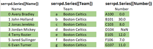
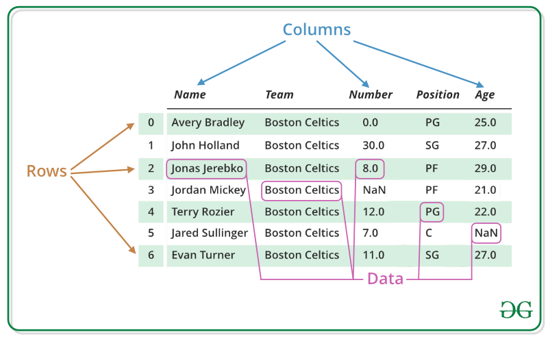
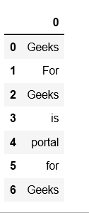

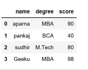


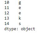
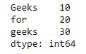
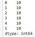
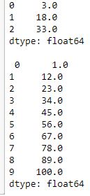

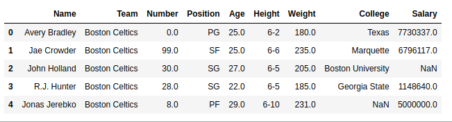
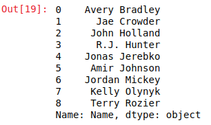
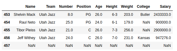
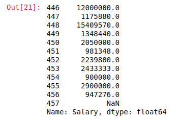

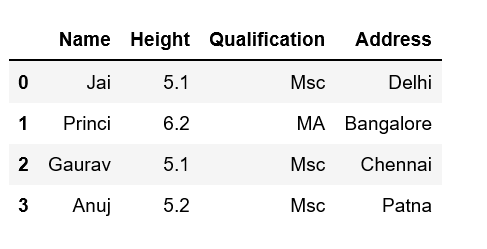
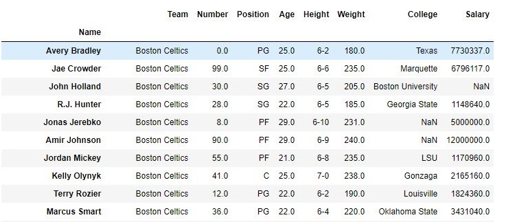
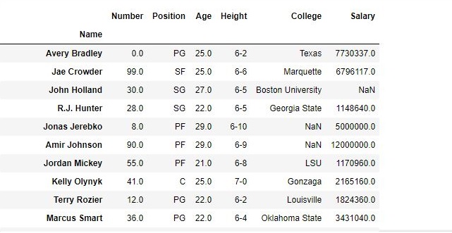
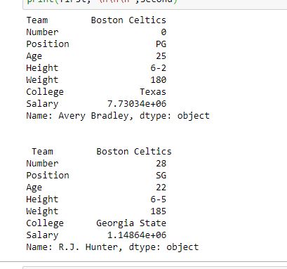
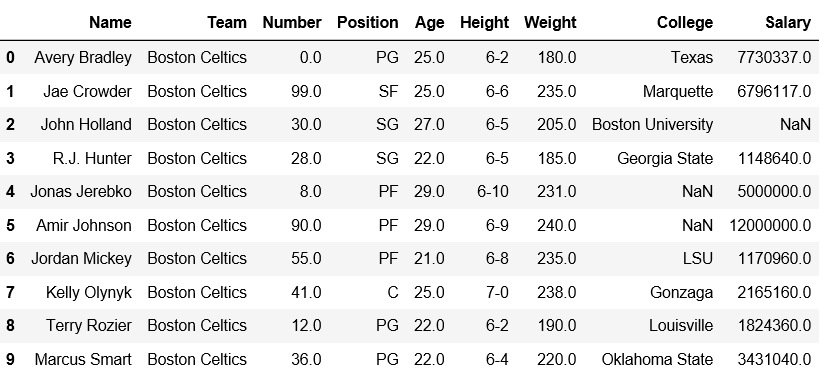
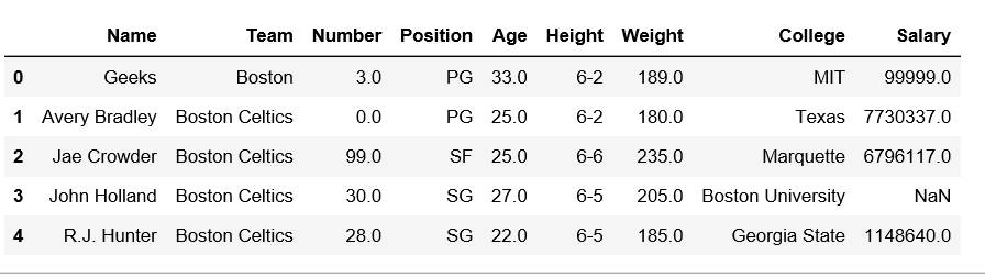
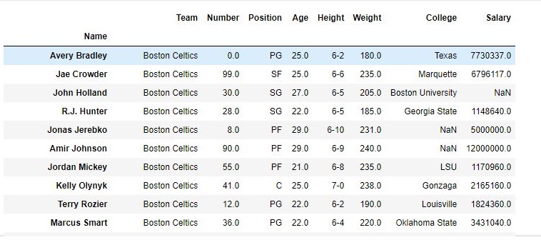
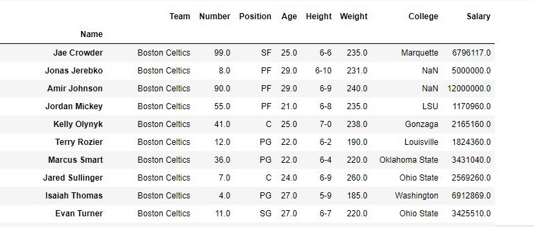
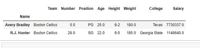
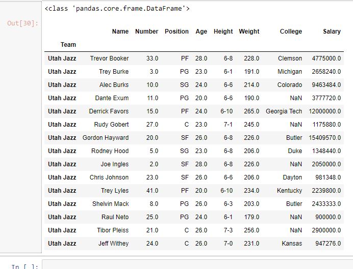
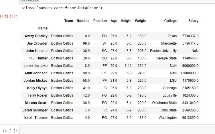
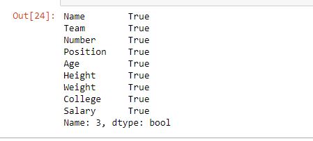
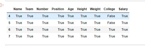
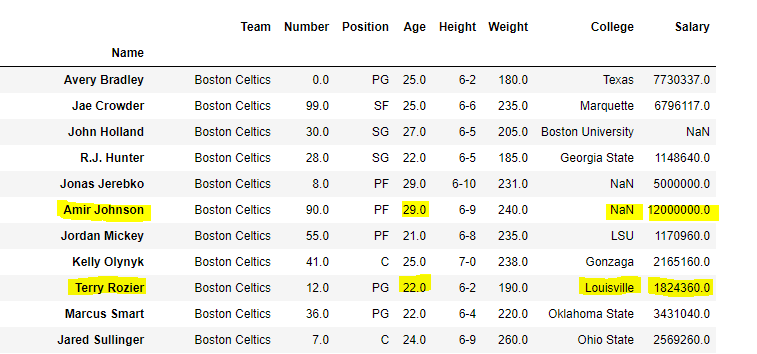
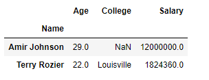
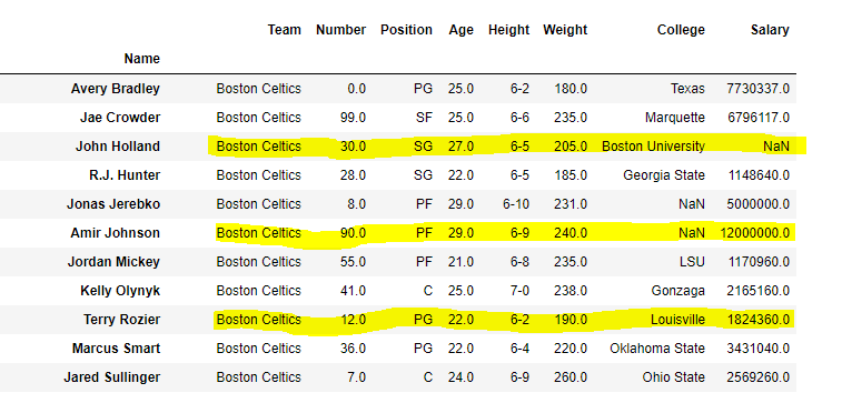
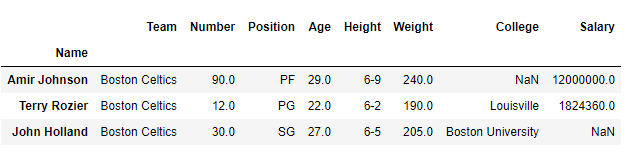
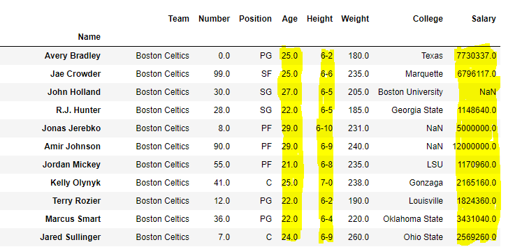
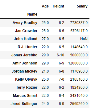
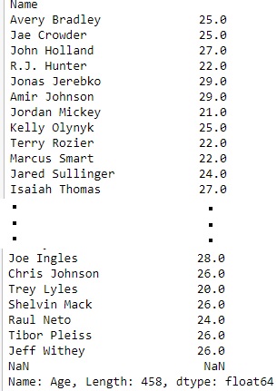
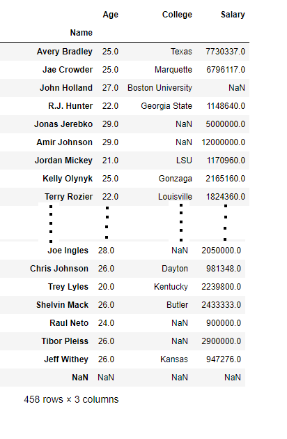
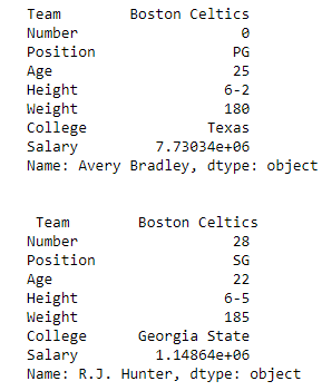
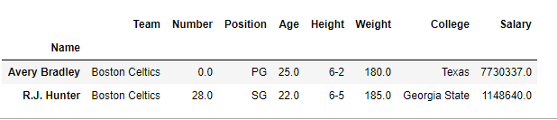

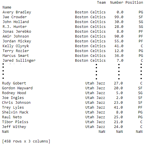
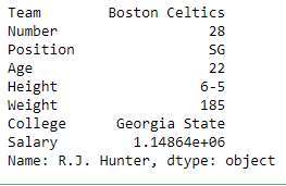
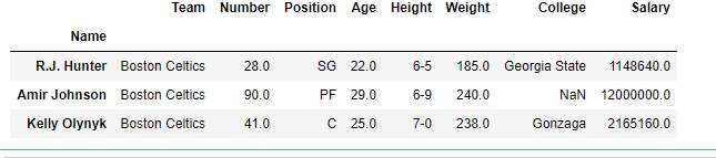
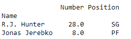
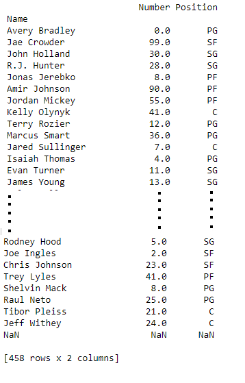
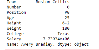
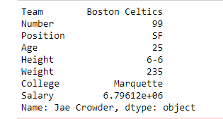


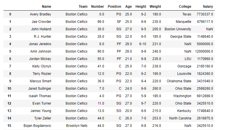
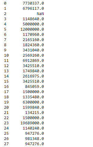
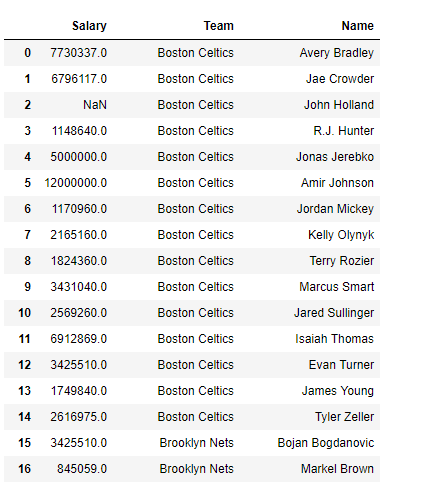


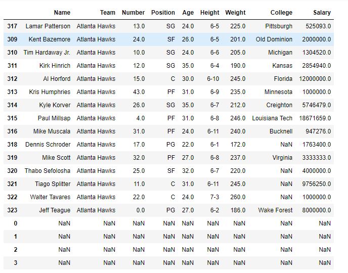

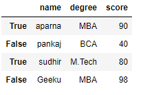
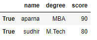
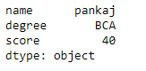
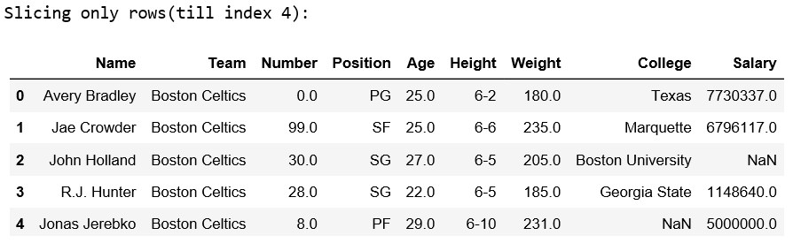
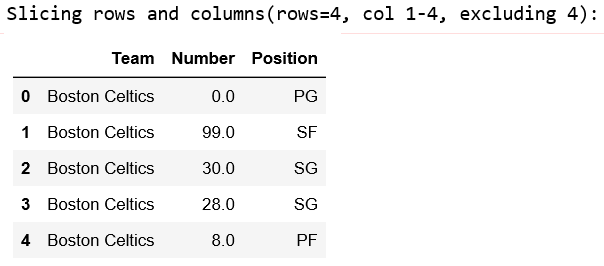
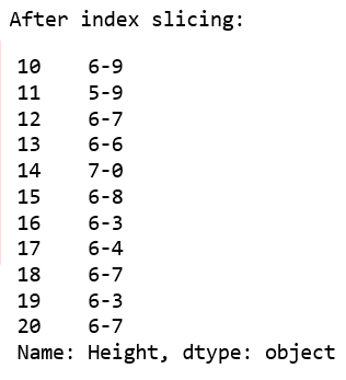
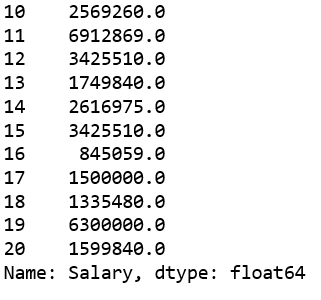
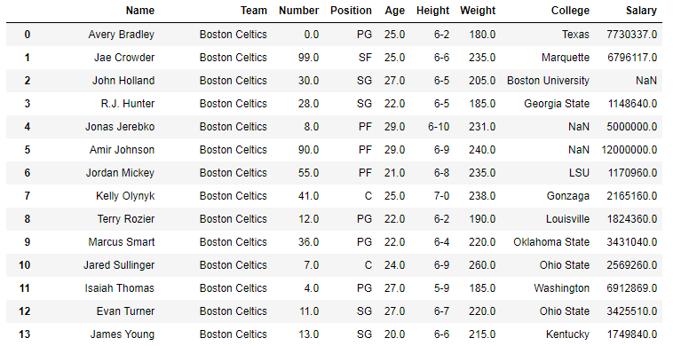


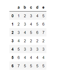
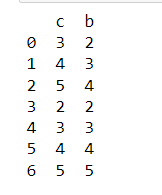
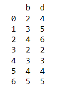
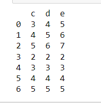
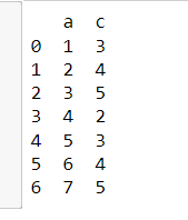
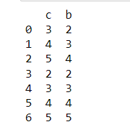
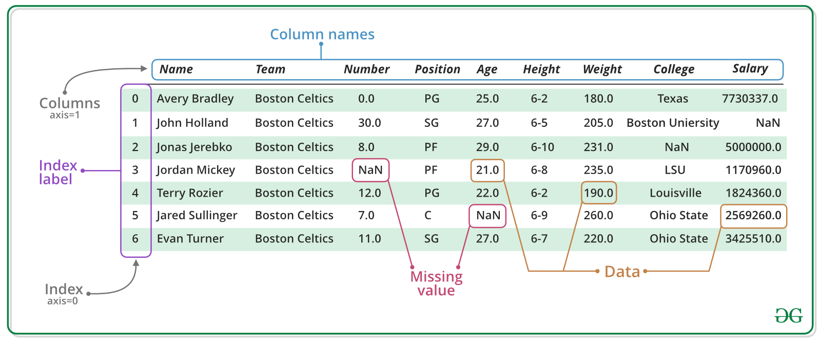
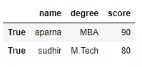
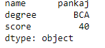
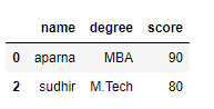
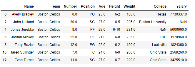
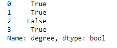
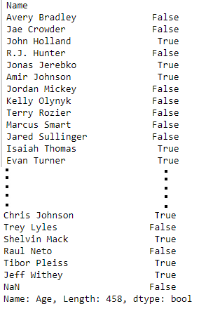
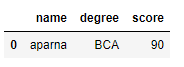
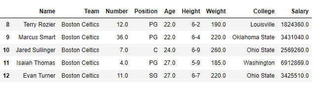
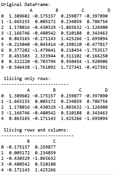
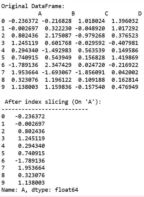
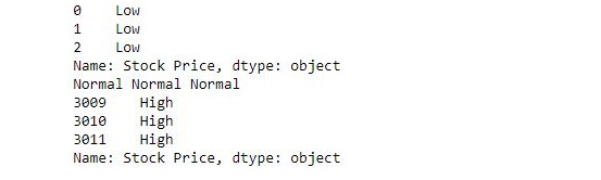
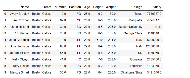
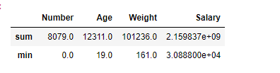
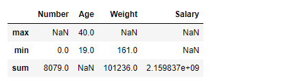
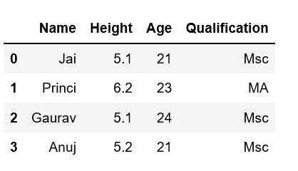
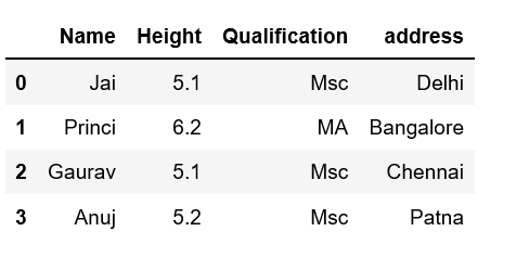
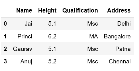
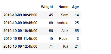
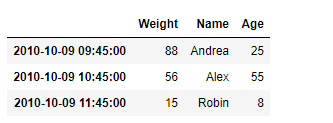
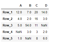
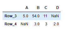
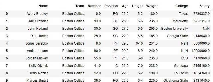
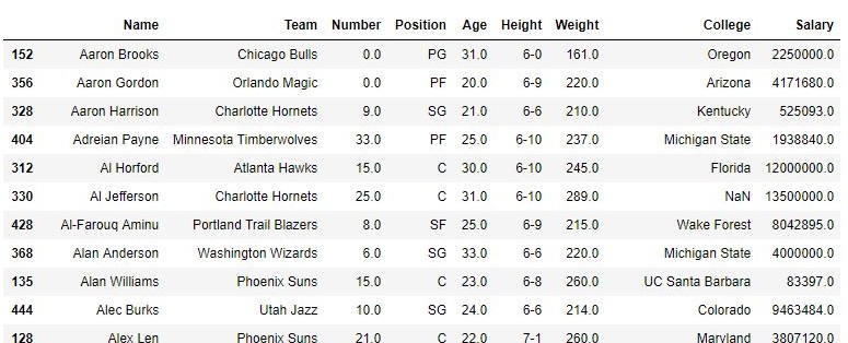
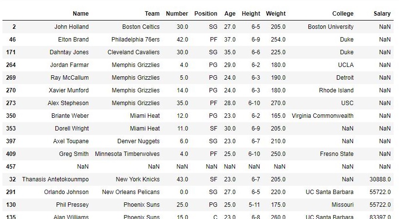
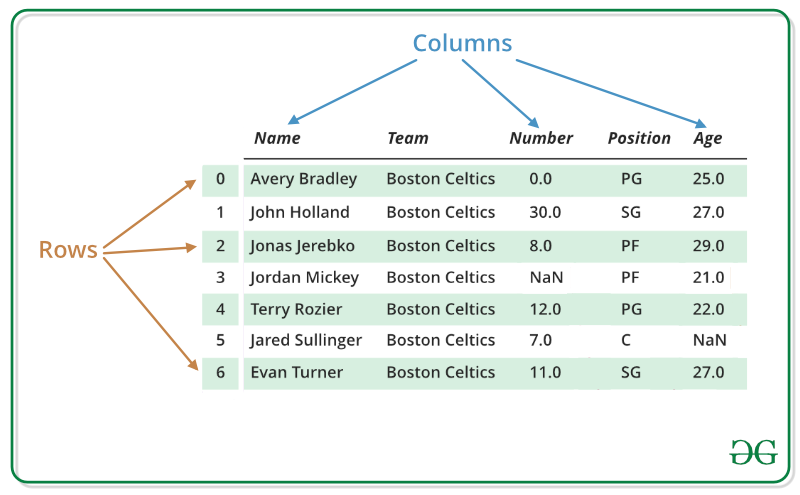


Comments
Post a Comment