https://docs.starburst.io/introduction/architecture.html

Starburst Enterprise platform (SEP) is a fast, interactive distributed SQL query engine that decouples compute from data storage. SEP lets you query data where it lives, including Hive, Snowflake, MySQL or even proprietary data stores.

NOT A DB, IS FEDERATED QUERY ENGINE.

is tool that enable fast and secure access to data across different source.

With Starburst as a single point of access and Immuta as a single point of access control, data teams can optimize performance and streamline self-service data access from a centralized access control plane.Built on trino.

Trino (formerly Presto® SQL) is the fastest open source, massively parallel processing SQL query engine designed for analytics of large datasets distributed over one or more data sources in object storage, databases and other systems.

A query engine is a system designed to receive queries, process them, and return results to the users.

An object storage system is a data source that stores data in files that live in a directory structure, rather than a relational database. Some common examples of object storage systems include Amazon S3 and Azure Data Lake Storage (ADLS).

architecture

At their heart, Starburst Enterprise and Starburst Galaxy are massively parallel processing (MPP) compute clusters running the distributed SQL query engine, Trino.

A cluster sits between a user’s favorite SQL client, and the existing data sources that they want to query. Data sources are represented by catalogs, and those catalogs specify the data source connectivity that the cluster needs to query the data sources. With Starburst products, you can query any connected data source.

A Trino cluster has two node types:

Coordinator - a single server that handles incoming queries, and provides query parsing and analysis, scheduling and planning. Distributes processing to worker nodes.
Workers - servers that execute tasks as directed by the coordinator, including retrieving data from the data source and processing data.

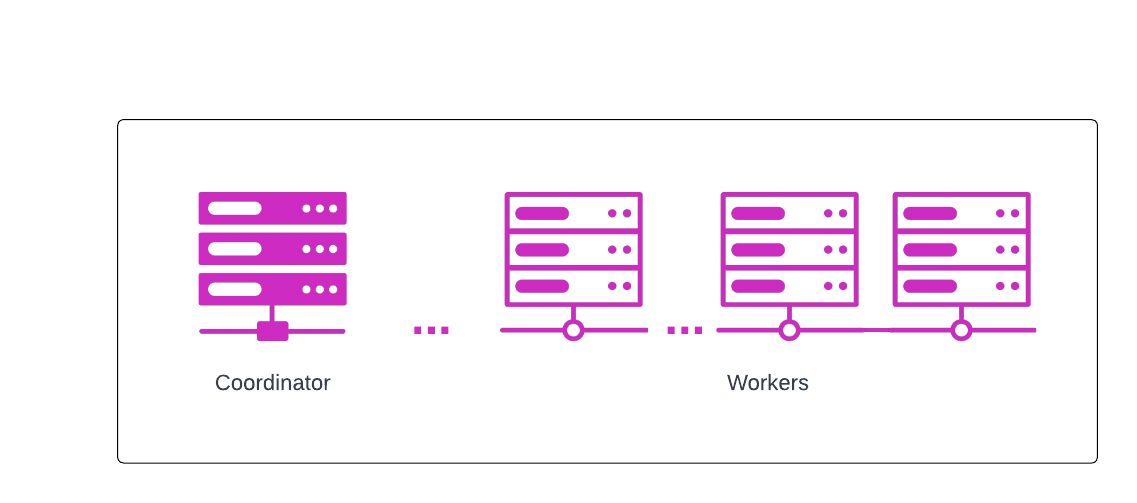
A single server process is run on each node in the cluster; only one node is designated as the coordinator. Worker nodes allow Starburst products to scale horizontally; more worker nodes means more processing resources. You can also scale up by increasing the size of the worker nodes,

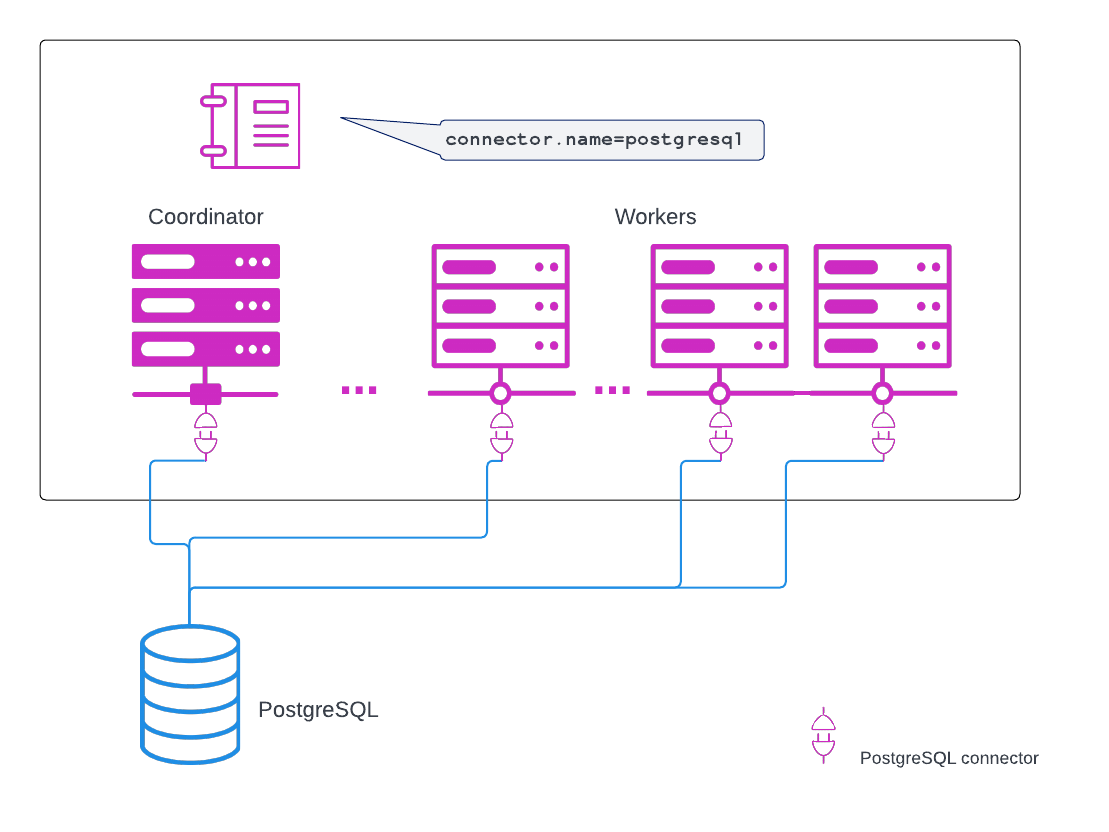
Rounding out Trino-based architecture is our suite of connectors. Connectors are what allow Starburst products to separate compute from storage. The configuration necessary to access a data source is called a catalog. Each catalog is configured with the connector for that particular data source. A connector is called when a catalog that is configured to use the connector is used in a query. Data source connections are established based on catalog configuration. The following example shows how this works with PostgreSQL, however, all RDBMS data sources are similarly configured:

Catalogs #

A catalog is the configuration that enables access to a specific data sources. Every cluster can have numerous catalogs configured, and therefore allow access to many data sources.

List all configured and available catalogs with the SQL statement SHOW CATALOGS (Galaxy / SEP ) in the Trino CLI or any other client:

SHOW CATALOGS;
 Catalog
---------
 hive_sales
 mysql_crm
(2 rows)

The query editor and other client tools also display a list of catalogs.

Connectors #

A connector is specific to the data source it supports. It transforms the underlying data into the SQL concepts of schemas, tables, columns, rows, and data types.

Connectors provide the following between a data source and Starburst Enterprise or Starburst Galaxy:

Secure communications link
Translation of data types
Handling of variances in the SQL implementation, adaption to a provided API, or translation of data in raw files

Every catalog uses a specific connector. Connectors are built-in features.

In SEP, you must specify a connector to create a catalog. In Starburst Galaxy, you create a catalog and the connector selection and configuration is handled for you.

Schemas #

Every catalog includes one or more schemas. They group together objects. Schemas are often equivalent to a specific database or schema in the underlying data source.

List all available schema in a specific catalog with the SQL statement SHOW SCHEMAS (Galaxy / SEP ) in the Trino CLI or any other client:

SHOW SCHEMA FROM examplecatalog;

Objects #

Every schema includes one or more objects. Typically these objects are tables.

List all available tables in a specific schema with the SQL statement SHOW TABLES (Galaxy / SEP ) in the Trino CLI or any other client:

SHOW TABLES FROM examplecatalog.exampleschema;

Some catalogs also support views and materialized views as objects.

More information about a table is available with the SQL statement SHOW COLUMNS (Galaxy / SEP ):

SHOW COLUMNS FROM examplecatalog.exampleschema.exampletable;

This information includes the columns in the table, the data type of the columns and other information.

Context #

The default context for any SQL statement is the catalog level. As a result any query to access a table needs to specific the catalog, schema and table establishing a fully-qualified name.

SELECT * FROM <catalog>.<schema>.<object>

This allows identical table names in the underlying data sources to be addressed specifically. The following to queries access tables of the same name in completely separate data sources:

SELECT * FROM sales.apac.customer;
SELECT * FROM marketing.americas.users;

Querying from multiple catalogs #

Starburst Enterprise and Starburst Galaxy let data consumers query anything, anywhere, and get the data they need in a single query. Specifically, they support queries that combine data from many different data sources at the same time.

Fully-qualified object names are critical when querying from multiple sources:

SELECT * FROM <catalog>.<schema>.<object>;

Here’s an example of data from two different sources, Hive and MySQL, combined into a single query:

SELECT
    sfm.account_number
FROM
    hive_sales.order_entries.orders oeo
JOIN
    mysql_crm.sf_history.customer_master sfm
ON sfm.account_number = oeo.customer_id
WHERE sfm.sf_industry = `medical` AND oeo.order_total > 300
LIMIT 2;

This query uses data from the following sources:

The orders table in the order_entries schema, which is defined in the hive_sales catalog
The customer_master table in the sf_history schema, which is defined in the mysql_crm catalog

Data lakes #

Modern businesses analyze and consume tremendous amounts of data, and modern data architecture has evolved to meet these business needs. Traditional data warehousing architectures struggle to keep up with the rate that businesses need to ingest and consume data.

A data lake is an architecture that allows your data to live in whatever format, software, or geographic region it currently resides in. This frees your data from vendor lock-in and removes the need for lengthy ETL processes that slow your business’s time-to-insight.

Architecture #

The modern data lake incorporates data transformation and governance in front of the lake, and is best described as a data lakehouse. The following diagram describes an example of data lakehouse architecture:

In this architecture, your data lives in whatever software, format, and location it needs in order to be most cost-effective on the lake. On top of this data storage layer, the lakehouse incorporates a data transformation layer that employs governance, materialized views, and other technologies and rules to ensure that the resulting data is ready for consumption.

The optimized data is then ready to be accessed by clients and BI tools through a query engine which handles data-level security, view management, and query optimization regardless of where in the lake the underlying data is stored.

Starburst for the data lake #

Starburst Galaxy and Starburst Enterprise platform (SEP) are ideal tools to get the most value out of your data lakehouse, with features to support scaling, optionality, high performance, and ease of data consumption.

Scaling and optionality #

Starburst products are designed to work in parallel with your data lakehouse, not lock your data into a restrictive, vendor-compliant architecture that increases costs and holds back your operational growth. Starburst products accomplish this with the following features:

Flexibility to access a wide variety of data sources.
Standard JDBC/ODBC drivers that allow connections to Starburst from many client and BI tools.
Cloud-friendly cluster architecture that separates computational resources from storage, allowing for flexible growth in whatever way best suits your operational needs.
Multi-cluster deployment options to handle cross-region workloads.

High performance #

Starburst products include a high-performing query engine out of the box, with the following features that support the most efficient use of your data lakehouse:

Query planning that distributes workloads across cluster resources, and pushing optimizations down to data sources to improve both processing speeds and network utilization.
Options to materialize data on the lake for high-speed access to data independent of performance on the data source.
High-performance I/O with multiple parallel connections between Starburst cluster nodes and object storage.
Object store caching and indexing to dynamically accelerate access to your lakehouse data.

Ease of consumption #

Starburst products are a central access point between your data consumers and your data lakehouse, streamlining access to the data most relevant to your users with the following features:

Centralized access control role and attribute-based access control (RBAC/ABAC) systems per-product that dictate persona-based access to your data.
Data product management that adds a semantic layer to your data for simplified consumption and sharing.
Support for modern BI tools and clients, allowing for organization-wide sharing and utilization of data insights.

Object storage fundamentals #

Rather than a traditional relational database, data in object storage systems is stored in a series of files that live in nested directories. These files can then be accessed with a query language using data warehouse systems like Hive. Some examples of object storage systems include the following:

Apache Hadoop Distributed File System (HDFS)
Amazon S3
Azure Data Lake Storage (ADLS)
Google Cloud Storage (GCS)
S3-compatible systems such as MinIO

The data files typically use one of the following supported binary formats:

ORC
Parquet
AVRO

Security

There are three main types of security measures for Starburst’s Trino-based clusters:

User authentication and client security
Security inside the cluster
Security between the cluster and data sources

Data transfers between the coordinator and workers inside the cluster use REST-based interactions over HTTP/HTTPS. Data transfers between clients and the cluster, and between the cluster and data sources, can also communicate securely via TLS and through REST-based APIs.

User authentication and client security #

Trino-based clusters allow you to authenticate users as they connect through their favorite client.

Clients communicate only with the cluster coordinator via a REST-like API, which can be configured to use TLS.

Authentication #

User authentication in Starburst Galaxy clusters is handled exclusively through the platform itself, which is managed in the Starburst Galaxy UI.

In Starburst Enterprise, authentication can be handled using one or more of the following authentication types:

LDAP
OAuth2
Okta
Salesforce
Password files
Certificates
JWT
Kerberos

How does this work? #

Data platforms in your organization such as Snowflake, Postgres, and Hive are defined by data engineers as catalogs. Catalogs, in turn, define schemas and their tables. Depending on the data access controls in place, discovering what data catalogs are available to you across all of your data platforms can be easy! Even through a CLI, it’s a single, simple query to get you started with your federated data:

trino> SHOW CATALOGS;
 Catalog
---------
 hive_sales
 mysql_crm
(2 rows)

After that, you can easily explore schemas in a catalog with the familiar SHOW SCHEMAS command:

trino> SHOW SCHEMAS FROM hive_sales LIKE `%rder%`;
 Schema
---------
 order_entries
 customer_orders
(2 rows)

From there, you can of course see the tables you might want to query:

trino> SHOW TABLES FROM order_entries;
 Table
-------
 orders
 order_items
(2 rows)

You might notice that even though you know from experience that some of your data is in MySQL and others in Hive, they all show up in the unified SHOW CATALOGS results. From here, you can simply join the data sources from different platforms as if they were from different tables. You just need to use their fully qualified names:

trino> SELECT
    sfm.account_number
FROM
    hive_sales.order_entries.orders oeo
JOIN
    mysql_crm.sf_history.customer_master sfm
ON sfm.account_number = oeo.customer_id
WHERE sfm.sf_industry = `medical` AND oeo.order_total > 300
LIMIT 2;

How do I get started? #

To begin, get the latest Starburst JDBC or ODBC driver and get it installed. Note that even though you very likely already have a JDBC or ODBC driver installed for your work, you do need the Starburst-specific driver. Be careful not to install either in the same directory with other JDBC or ODBC drivers.

If your data ops group has not already given you the required connection information, reach out to them for the following:

the JDBC URL - jdbc:trino://example.net:8080
whether your org is using SSL to connect
the type of authentication your org is using - username or LDAP

When you have that info and your driver is installed, you are ready to connect.

What kind of tools can I use? #

More than likely, you can use all your client tools, and even ones on your wishlist with the the help of the Clients section of our documentation.

CALL

Call a procedure using positional arguments:

CALL test(123, 'apple');

Call a procedure using named arguments:

CALL test(name => 'apple', id => 123);

Call a procedure using a fully qualified name:

CALL catalog.schema.test();

DEALLOCATE PREPARE#

Synopsis#

DEALLOCATE PREPARE statement_name

Description#

Removes a statement with the name statement_name from the list of prepared statements in a session.

Examples#

Deallocate a statement with the name my_query:

DEALLOCATE PREPARE my_query;

DESCRIBE INPUT#

Synopsis#

DESCRIBE INPUT statement_name

Description#

Lists the input parameters of a prepared statement along with the position and type of each parameter. Parameter types that cannot be determined will appear as unknown.

Examples#

Prepare and describe a query with three parameters:

PREPARE my_select1 FROM
SELECT ? FROM nation WHERE regionkey = ? AND name < ?;

DESCRIBE INPUT my_select1;

 Position | Type
--------------------
        0 | unknown
        1 | bigint
        2 | varchar
(3 rows)

Prepare and describe a query with no parameters:

PREPARE my_select2 FROM
SELECT * FROM nation;

DESCRIBE INPUT my_select2;

 Position | Type
-----------------
(0 rows)

DESCRIBE OUTPUT#

Synopsis#

DESCRIBE OUTPUT statement_name

Description#

List the output columns of a prepared statement, including the column name (or alias), catalog, schema, table, type, type size in bytes, and a boolean indicating if the column is aliased.

Examples#

Prepare and describe a query with four output columns:

PREPARE my_select1 FROM
SELECT * FROM nation;

DESCRIBE OUTPUT my_select1;

 Column Name | Catalog | Schema | Table  |  Type   | Type Size | Aliased
-------------+---------+--------+--------+---------+-----------+---------
 nationkey   | tpch    | sf1    | nation | bigint  |         8 | false
 name        | tpch    | sf1    | nation | varchar |         0 | false
 regionkey   | tpch    | sf1    | nation | bigint  |         8 | false
 comment     | tpch    | sf1    | nation | varchar |         0 | false
(4 rows)

EXECUTE#

Synopsis#

EXECUTE statement_name [ USING parameter1 [ , parameter2, ... ] ]

Description#

Executes a prepared statement with the name `statement_name`. Parameter values are defined in the `USING` clause.

Examples#

Prepare and execute a query with no parameters:

PREPARE my_select1 FROM
SELECT name FROM nation;

EXECUTE my_select1;

Prepare and execute a query with two parameters:

PREPARE my_select2 FROM
SELECT name FROM nation WHERE regionkey = ? and nationkey < ?;

EXECUTE my_select2 USING 1, 3;

This is equivalent to:

SELECT name FROM nation WHERE regionkey = 1 AND nationkey < 3;

EXECUTE IMMEDIATE#

Synopsis#

EXECUTE IMMEDIATE `statement` [ USING parameter1 [ , parameter2, ... ] ]

Description#

Executes a statement without the need to prepare or deallocate the statement. Parameter values are defined in the `USING` clause.

Examples#

Execute a query with no parameters:

EXECUTE IMMEDIATE
'SELECT name FROM nation';

Execute a query with two parameters:

EXECUTE IMMEDIATE
'SELECT name FROM nation WHERE regionkey = ? and nationkey < ?'
USING 1, 3;

This is equivalent to:

PREPARE statement_name FROM SELECT name FROM nation WHERE regionkey = ? and nationkey < ?
EXECUTE statement_name USING 1, 3
DEALLOCATE PREPARE statement_name

EXPLAIN#

Synopsis#

EXPLAIN [ ( option [, ...] ) ] statement

where option can be one of:

FORMAT { TEXT | GRAPHVIZ | JSON }
TYPE { LOGICAL | DISTRIBUTED | VALIDATE | IO }

Description#

Show the logical or distributed execution plan of a statement, or validate the statement. The distributed plan is shown by default. Each plan fragment of the distributed plan is executed by a single or multiple Trino nodes. Fragments separation represent the data exchange between Trino nodes. Fragment type specifies how the fragment is executed by Trino nodes and how the data is distributed between fragments:
`SINGLE`
Fragment is executed on a single node.
`HASH`
Fragment is executed on a fixed number of nodes with the input data distributed using a hash function.
`ROUND_ROBIN`
Fragment is executed on a fixed number of nodes with the input data distributed in a round-robin fashion.
`BROADCAST`
Fragment is executed on a fixed number of nodes with the input data broadcasted to all nodes.
`SOURCE`
Fragment is executed on nodes where input splits are accessed.

Examples#

EXPLAIN (TYPE LOGICAL)#

Process the supplied query statement and create a logical plan in text format:

EXPLAIN (TYPE LOGICAL) SELECT regionkey, count(*) FROM nation GROUP BY 1;

PREPARE#

Synopsis#

PREPARE statement_name FROM statement

Description#

Prepares a statement for execution at a later time. Prepared statements are queries that are saved in a session with a given name. The statement can include parameters in place of literals to be replaced at execution time. Parameters are represented by question marks.

Examples#

Prepare a select query:

PREPARE my_select1 FROM
SELECT * FROM nation;

Prepare a select query that includes parameters. The values to compare with regionkey and nationkey will be filled in with the EXECUTE statement:

PREPARE my_select2 FROM
SELECT name FROM nation WHERE regionkey = ? AND nationkey < ?;

Prepare an insert query:

PREPARE my_insert FROM
INSERT INTO cities VALUES (1, 'San Francisco');

SHOW FUNCTIONS#

Synopsis#

SHOW FUNCTIONS [ LIKE pattern ]

Description#

List all the functions available for use in queries. For each function returned, the following information is displayed:

Function name
Return type
Argument types
Function type
Deterministic
Description

Specify a pattern in the optional LIKE clause to filter the results to the desired subset. For example, the following query allows you to find functions beginning with array:

SHOW FUNCTIONS LIKE 'array%';

USE#

Synopsis#

USE catalog.schema
USE schema

Description#

Update the session to use the specified catalog and schema. If a catalog is not specified, the schema is resolved relative to the current catalog.

Examples#

USE hive.finance;
USE information_schema;

VALUES#

Synopsis#

VALUES row [, ...]

where row is a single expression or

( column_expression [, ...] )

Description#

Defines a literal inline table.

VALUES can be used anywhere a query can be used (e.g., the FROM clause of a SELECT, an INSERT, or even at the top level). VALUES creates an anonymous table without column names, but the table and columns can be named using an AS clause with column aliases.

Examples#

Return a table with one column and three rows:

VALUES 1, 2, 3

Return a table with two columns and three rows:

VALUES
    (1, 'a'),
    (2, 'b'),
    (3, 'c')

Return table with column id and name:

SELECT * FROM (
    VALUES
        (1, 'a'),
        (2, 'b'),
        (3, 'c')
) AS t (id, name)

Create a new table with column id and name:

CREATE TABLE example AS
SELECT * FROM (
    VALUES
        (1, 'a'),
        (2, 'b'),
        (3, 'c')
) AS t (id, name)

SELECT#

Synopsis#

[ WITH [ RECURSIVE ] with_query [, ...] ]
SELECT [ ALL | DISTINCT ] select_expression [, ...]
[ FROM from_item [, ...] ]
[ WHERE condition ]
[ GROUP BY [ ALL | DISTINCT ] grouping_element [, ...] ]
[ HAVING condition]
[ WINDOW window_definition_list]
[ { UNION | INTERSECT | EXCEPT } [ ALL | DISTINCT ] select ]
[ ORDER BY expression [ ASC | DESC ] [, ...] ]
[ OFFSET count [ ROW | ROWS ] ]
[ LIMIT { count | ALL } ]
[ FETCH { FIRST | NEXT } [ count ] { ROW | ROWS } { ONLY | WITH TIES } ]

where from_item is one of

table_name [ [ AS ] alias [ ( column_alias [, ...] ) ] ]

from_item join_type from_item
  [ ON join_condition | USING ( join_column [, ...] ) ]

table_name [ [ AS ] alias [ ( column_alias [, ...] ) ] ]
  MATCH_RECOGNIZE pattern_recognition_specification
    [ [ AS ] alias [ ( column_alias [, ...] ) ] ]

For detailed description of MATCH_RECOGNIZE clause, see pattern recognition in FROM clause.

TABLE (table_function_invocation) [ [ AS ] alias [ ( column_alias [, ...] ) ] ]

For description of table functions usage, see table functions.

and join_type is one of

[ INNER ] JOIN
LEFT [ OUTER ] JOIN
RIGHT [ OUTER ] JOIN
FULL [ OUTER ] JOIN
CROSS JOIN

and grouping_element is one of

()
expression
GROUPING SETS ( ( column [, ...] ) [, ...] )
CUBE ( column [, ...] )
ROLLUP ( column [, ...] )

Description#

Retrieve rows from zero or more tables.

WITH clause#

The WITH clause defines named relations for use within a query. It allows flattening nested queries or simplifying subqueries. This also works with multiple subqueries:

WITH
  t1 AS (SELECT a, MAX(b) AS b FROM x GROUP BY a),
  t2 AS (SELECT a, AVG(d) AS d FROM y GROUP BY a)
SELECT t1.*, t2.*
FROM t1
JOIN t2 ON t1.a = t2.a;

Additionally, the relations within a WITH clause can chain:

WITH
  x AS (SELECT a FROM t),
  y AS (SELECT a AS b FROM x),
  z AS (SELECT b AS c FROM y)
SELECT c FROM z;

Warning

Currently, the SQL for the WITH clause will be inlined anywhere the named relation is used. This means that if the relation is used more than once and the query is non-deterministic, the results may be different each time.

WITH RECURSIVE clause#

The WITH RECURSIVE clause is a variant of the WITH clause. It defines a list of queries to process, including recursive processing of suitable queries.

Warning

This feature is experimental only. Proceed to use it only if you understand potential query failures and the impact of the recursion processing on your workload.

A recursive WITH-query must be shaped as a UNION of two relations. The first relation is called the recursion base, and the second relation is called the recursion step. Trino supports recursive WITH-queries with a single recursive reference to a WITH-query from within the query. The name T of the query T can be mentioned once in the FROM clause of the recursion step relation.

The following listing shows a simple example, that displays a commonly used form of a single query in the list:

WITH RECURSIVE t(n) AS (
    VALUES (1)
    UNION ALL
    SELECT n + 1 FROM t WHERE n < 4
)
SELECT sum(n) FROM t;

In the preceding query the simple assignment VALUES (1) defines the recursion base relation. SELECT n + 1 FROM t WHERE n < 4 defines the recursion step relation. The recursion processing performs these steps:

recursive base yields 1
first recursion yields 1 + 1 = 2
second recursion uses the result from the first and adds one: 2 + 1 = 3
third recursion uses the result from the second and adds one again: 3 + 1 = 4
fourth recursion aborts since n = 4
this results in t having values 1, 2, 3 and 4
the final statement performs the sum operation of these elements with the final result value 10

The types of the returned columns are those of the base relation. Therefore it is required that types in the step relation can be coerced to base relation types.

The RECURSIVE clause applies to all queries in the WITH list, but not all of them must be recursive. If a WITH-query is not shaped according to the rules mentioned above or it does not contain a recursive reference, it is processed like a regular WITH-query. Column aliases are mandatory for all the queries in the recursive WITH list.

The following limitations apply as a result of following the SQL standard and due to implementation choices, in addition to WITH clause limitations:

only single-element recursive cycles are supported. Like in regular WITH-queries, references to previous queries in the WITH list are allowed. References to following queries are forbidden.
usage of outer joins, set operations, limit clause, and others is not always allowed in the step relation
recursion depth is fixed, defaults to 10, and doesn’t depend on the actual query results

You can adjust the recursion depth with the session property max_recursion_depth. When changing the value consider that the size of the query plan growth is quadratic with the recursion depth.

If column aliases are specified, they override any preexisting column or row field names:

SELECT (CAST(ROW(1, true) AS ROW(field1 bigint, field2 boolean))).* AS (alias1, alias2);

 alias1 | alias2
--------+--------
      1 | true
(1 row)

Otherwise, the existing names are used:

SELECT (CAST(ROW(1, true) AS ROW(field1 bigint, field2 boolean))).*;

 field1 | field2
--------+--------
      1 | true
(1 row)

and in their absence, anonymous columns are produced:

SELECT (ROW(1, true)).*;

 _col0 | _col1
-------+-------
     1 | true
(1 row)

GROUP BY clause#

The GROUP BY clause divides the output of a SELECT statement into groups of rows containing matching values. A simple GROUP BY clause may contain any expression composed of input columns or it may be an ordinal number selecting an output column by position (starting at one).

The following queries are equivalent. They both group the output by the nationkey input column with the first query using the ordinal position of the output column and the second query using the input column name:

SELECT count(*), nationkey FROM customer GROUP BY 2;

SELECT count(*), nationkey FROM customer GROUP BY nationkey;

GROUP BY clauses can group output by input column names not appearing in the output of a select statement. For example, the following query generates row counts for the customer table using the input column mktsegment:

SELECT count(*) FROM customer GROUP BY mktsegment;

 _col0
-------
 29968
 30142
 30189
 29949
 29752
(5 rows)

When a GROUP BY clause is used in a SELECT statement all output expressions must be either aggregate functions or columns present in the GROUP BY clause.

Complex grouping operations#

Trino also supports complex aggregations using the `GROUPING SETS`, `CUBE` and `ROLLUP` syntax. This syntax allows users to perform analysis that requires aggregation on multiple sets of columns in a single query. Complex grouping operations do not support grouping on expressions composed of input columns. Only column names are allowed.
Complex grouping operations are often equivalent to a `UNION ALL` of simple `GROUP BY` expressions, as shown in the following examples. This equivalence does not apply, however, when the source of data for the aggregation is non-deterministic.

GROUPING SETS#

Grouping sets allow users to specify multiple lists of columns to group on. The columns not part of a given sublist of grouping columns are set to NULL.

SELECT * FROM shipping;

 origin_state | origin_zip | destination_state | destination_zip | package_weight
--------------+------------+-------------------+-----------------+----------------
 California   |      94131 | New Jersey        |            8648 |             13
 California   |      94131 | New Jersey        |            8540 |             42
 New Jersey   |       7081 | Connecticut       |            6708 |            225
 California   |      90210 | Connecticut       |            6927 |           1337
 California   |      94131 | Colorado          |           80302 |              5
 New York     |      10002 | New Jersey        |            8540 |              3
(6 rows)

GROUPING SETS semantics are demonstrated by this example query:

SELECT origin_state, origin_zip, destination_state, sum(package_weight)
FROM shipping
GROUP BY GROUPING SETS (
    (origin_state),
    (origin_state, origin_zip),
    (destination_state));

 origin_state | origin_zip | destination_state | _col0
--------------+------------+-------------------+-------
 New Jersey   | NULL       | NULL              |   225
 California   | NULL       | NULL              |  1397
 New York     | NULL       | NULL              |     3
 California   |      90210 | NULL              |  1337
 California   |      94131 | NULL              |    60
 New Jersey   |       7081 | NULL              |   225
 New York     |      10002 | NULL              |     3
 NULL         | NULL       | Colorado          |     5
 NULL         | NULL       | New Jersey        |    58
 NULL         | NULL       | Connecticut       |  1562
(10 rows)

The preceding query may be considered logically equivalent to a UNION ALL of multiple GROUP BY queries:

SELECT origin_state, NULL, NULL, sum(package_weight)
FROM shipping GROUP BY origin_state

UNION ALL

SELECT origin_state, origin_zip, NULL, sum(package_weight)
FROM shipping GROUP BY origin_state, origin_zip

UNION ALL

SELECT NULL, NULL, destination_state, sum(package_weight)
FROM shipping GROUP BY destination_state;

However, the query with the complex grouping syntax (GROUPING SETS, CUBE or ROLLUP) will only read from the underlying data source once, while the query with the UNION ALL reads the underlying data three times. This is why queries with a UNION ALL may produce inconsistent results when the data source is not deterministic.

CUBE#

The CUBE operator generates all possible grouping sets (i.e. a power set) for a given set of columns. For example, the query:

SELECT origin_state, destination_state, sum(package_weight)
FROM shipping
GROUP BY CUBE (origin_state, destination_state);

is equivalent to:

SELECT origin_state, destination_state, sum(package_weight)
FROM shipping
GROUP BY GROUPING SETS (
    (origin_state, destination_state),
    (origin_state),
    (destination_state),
    ()
);

 origin_state | destination_state | _col0
--------------+-------------------+-------
 California   | New Jersey        |    55
 California   | Colorado          |     5
 New York     | New Jersey        |     3
 New Jersey   | Connecticut       |   225
 California   | Connecticut       |  1337
 California   | NULL              |  1397
 New York     | NULL              |     3
 New Jersey   | NULL              |   225
 NULL         | New Jersey        |    58
 NULL         | Connecticut       |  1562
 NULL         | Colorado          |     5
 NULL         | NULL              |  1625
(12 rows)

ROLLUP#

The ROLLUP operator generates all possible subtotals for a given set of columns. For example, the query:

SELECT origin_state, origin_zip, sum(package_weight)
FROM shipping
GROUP BY ROLLUP (origin_state, origin_zip);

 origin_state | origin_zip | _col2
--------------+------------+-------
 California   |      94131 |    60
 California   |      90210 |  1337
 New Jersey   |       7081 |   225
 New York     |      10002 |     3
 California   | NULL       |  1397
 New York     | NULL       |     3
 New Jersey   | NULL       |   225
 NULL         | NULL       |  1625
(8 rows)

is equivalent to:

SELECT origin_state, origin_zip, sum(package_weight)
FROM shipping
GROUP BY GROUPING SETS ((origin_state, origin_zip), (origin_state), ());

Combining multiple grouping expressions#

Multiple grouping expressions in the same query are interpreted as having cross-product semantics. For example, the following query:

SELECT origin_state, destination_state, origin_zip, sum(package_weight)
FROM shipping
GROUP BY
    GROUPING SETS ((origin_state, destination_state)),
    ROLLUP (origin_zip);

which can be rewritten as:

SELECT origin_state, destination_state, origin_zip, sum(package_weight)
FROM shipping
GROUP BY
    GROUPING SETS ((origin_state, destination_state)),
    GROUPING SETS ((origin_zip), ());

is logically equivalent to:

SELECT origin_state, destination_state, origin_zip, sum(package_weight)
FROM shipping
GROUP BY GROUPING SETS (
    (origin_state, destination_state, origin_zip),
    (origin_state, destination_state)
);

 origin_state | destination_state | origin_zip | _col3
--------------+-------------------+------------+-------
 New York     | New Jersey        |      10002 |     3
 California   | New Jersey        |      94131 |    55
 New Jersey   | Connecticut       |       7081 |   225
 California   | Connecticut       |      90210 |  1337
 California   | Colorado          |      94131 |     5
 New York     | New Jersey        | NULL       |     3
 New Jersey   | Connecticut       | NULL       |   225
 California   | Colorado          | NULL       |     5
 California   | Connecticut       | NULL       |  1337
 California   | New Jersey        | NULL       |    55
(10 rows)

The ALL and DISTINCT quantifiers determine whether duplicate grouping sets each produce distinct output rows. This is particularly useful when multiple complex grouping sets are combined in the same query. For example, the following query:

SELECT origin_state, destination_state, origin_zip, sum(package_weight)
FROM shipping
GROUP BY ALL
    CUBE (origin_state, destination_state),
    ROLLUP (origin_state, origin_zip);

is equivalent to:

SELECT origin_state, destination_state, origin_zip, sum(package_weight)
FROM shipping
GROUP BY GROUPING SETS (
    (origin_state, destination_state, origin_zip),
    (origin_state, origin_zip),
    (origin_state, destination_state, origin_zip),
    (origin_state, origin_zip),
    (origin_state, destination_state),
    (origin_state),
    (origin_state, destination_state),
    (origin_state),
    (origin_state, destination_state),
    (origin_state),
    (destination_state),
    ()
);

However, if the query uses the DISTINCT quantifier for the GROUP BY:

SELECT origin_state, destination_state, origin_zip, sum(package_weight)
FROM shipping
GROUP BY DISTINCT
    CUBE (origin_state, destination_state),
    ROLLUP (origin_state, origin_zip);

only unique grouping sets are generated:

SELECT origin_state, destination_state, origin_zip, sum(package_weight)
FROM shipping
GROUP BY GROUPING SETS (
    (origin_state, destination_state, origin_zip),
    (origin_state, origin_zip),
    (origin_state, destination_state),
    (origin_state),
    (destination_state),
    ()
);

The default set quantifier is ALL.

GROUPING operation#

grouping(col1, ..., colN) -> bigint

The grouping operation returns a bit set converted to decimal, indicating which columns are present in a grouping. It must be used in conjunction with GROUPING SETS, ROLLUP, CUBE or GROUP BY and its arguments must match exactly the columns referenced in the corresponding GROUPING SETS, ROLLUP, CUBE or GROUP BY clause.

To compute the resulting bit set for a particular row, bits are assigned to the argument columns with the rightmost column being the least significant bit. For a given grouping, a bit is set to 0 if the corresponding column is included in the grouping and to 1 otherwise. For example, consider the query below:

SELECT origin_state, origin_zip, destination_state, sum(package_weight),
       grouping(origin_state, origin_zip, destination_state)
FROM shipping
GROUP BY GROUPING SETS (
    (origin_state),
    (origin_state, origin_zip),
    (destination_state)
);

origin_state | origin_zip | destination_state | _col3 | _col4
--------------+------------+-------------------+-------+-------
California   | NULL       | NULL              |  1397 |     3
New Jersey   | NULL       | NULL              |   225 |     3
New York     | NULL       | NULL              |     3 |     3
California   |      94131 | NULL              |    60 |     1
New Jersey   |       7081 | NULL              |   225 |     1
California   |      90210 | NULL              |  1337 |     1
New York     |      10002 | NULL              |     3 |     1
NULL         | NULL       | New Jersey        |    58 |     6
NULL         | NULL       | Connecticut       |  1562 |     6
NULL         | NULL       | Colorado          |     5 |     6
(10 rows)

The first grouping in the above result only includes the origin_state column and excludes the origin_zip and destination_state columns. The bit set constructed for that grouping is 011 where the most significant bit represents origin_state.

HAVING clause#

The HAVING clause is used in conjunction with aggregate functions and the GROUP BY clause to control which groups are selected. A HAVING clause eliminates groups that do not satisfy the given conditions. HAVING filters groups after groups and aggregates are computed.

The following example queries the customer table and selects groups with an account balance greater than the specified value:

SELECT count(*), mktsegment, nationkey,
       CAST(sum(acctbal) AS bigint) AS totalbal
FROM customer
GROUP BY mktsegment, nationkey
HAVING sum(acctbal) > 5700000
ORDER BY totalbal DESC;

 _col0 | mktsegment | nationkey | totalbal
-------+------------+-----------+----------
  1272 | AUTOMOBILE |        19 |  5856939
  1253 | FURNITURE  |        14 |  5794887
  1248 | FURNITURE  |         9 |  5784628
  1243 | FURNITURE  |        12 |  5757371
  1231 | HOUSEHOLD  |         3 |  5753216
  1251 | MACHINERY  |         2 |  5719140
  1247 | FURNITURE  |         8 |  5701952
(7 rows)

WINDOW clause#

The WINDOW clause is used to define named window specifications. The defined named window specifications can be referred to in the SELECT and ORDER BY clauses of the enclosing query:

SELECT orderkey, clerk, totalprice,
      rank() OVER w AS rnk
FROM orders
WINDOW w AS (PARTITION BY clerk ORDER BY totalprice DESC)
ORDER BY count() OVER w, clerk, rnk

The window definition list of WINDOW clause can contain one or multiple named window specifications of the form

window_name AS (window_specification)

A window specification has the following components:

The existing window name, which refers to a named window specification in the WINDOW clause. The window specification associated with the referenced name is the basis of the current specification.
The partition specification, which separates the input rows into different partitions. This is analogous to how the GROUP BY clause separates rows into different groups for aggregate functions.
The ordering specification, which determines the order in which input rows will be processed by the window function.
The window frame, which specifies a sliding window of rows to be processed by the function for a given row. If the frame is not specified, it defaults to RANGE UNBOUNDED PRECEDING, which is the same as RANGE BETWEEN UNBOUNDED PRECEDING AND CURRENT ROW. This frame contains all rows from the start of the partition up to the last peer of the current row. In the absence of ORDER BY, all rows are considered peers, so RANGE BETWEEN UNBOUNDED PRECEDING AND CURRENT ROW is equivalent to BETWEEN UNBOUNDED PRECEDING AND UNBOUNDED FOLLOWING. The window frame syntax supports additional clauses for row pattern recognition. If the row pattern recognition clauses are specified, the window frame for a particular row consists of the rows matched by a pattern starting from that row. Additionally, if the frame specifies row pattern measures, they can be called over the window, similarly to window functions. For more details, see Row pattern recognition in window structures.

Each window component is optional. If a window specification does not specify window partitioning, ordering or frame, those components are obtained from the window specification referenced by the existing window name, or from another window specification in the reference chain. In case when there is no existing window name specified, or none of the referenced window specifications contains the component, the default value is used.

Set operations#

UNION INTERSECT and EXCEPT are all set operations. These clauses are used to combine the results of more than one select statement into a single result set:

query UNION [ALL | DISTINCT] query

query INTERSECT [ALL | DISTINCT] query

query EXCEPT [ALL | DISTINCT] query

The argument ALL or DISTINCT controls which rows are included in the final result set. If the argument ALL is specified all rows are included even if the rows are identical. If the argument DISTINCT is specified only unique rows are included in the combined result set. If neither is specified, the behavior defaults to DISTINCT.

Multiple set operations are processed left to right, unless the order is explicitly specified via parentheses. Additionally, INTERSECT binds more tightly than EXCEPT and UNION. That means A UNION B INTERSECT C EXCEPT D is the same as A UNION (B INTERSECT C) EXCEPT D.

This is the order of operations:

Expressions in parentheses.
The INTERSECT operator.
EXCEPT (equivalent of Oracle MINUS) and UNION evaluated from left to right based on their position in the expression.

UNION clause#

UNION combines all the rows that are in the result set from the first query with those that are in the result set for the second query. The following is an example of one of the simplest possible UNION clauses. It selects the value 13 and combines this result set with a second query that selects the value 42:

SELECT 13
UNION
SELECT 42;

 _col0
-------
    13
    42
(2 rows)

The following query demonstrates the difference between UNION and UNION ALL. It selects the value 13 and combines this result set with a second query that selects the values 42 and 13:

SELECT 13
UNION
SELECT * FROM (VALUES 42, 13);

 _col0
-------
    13
    42
(2 rows)

SELECT 13
UNION ALL
SELECT * FROM (VALUES 42, 13);

 _col0
-------
    13
    42
    13
(2 rows)

INTERSECT clause#

INTERSECT returns only the rows that are in the result sets of both the first and the second queries. The following is an example of one of the simplest possible INTERSECT clauses. It selects the values 13 and 42 and combines this result set with a second query that selects the value 13. Since 42 is only in the result set of the first query, it is not included in the final results.:

SELECT * FROM (VALUES 13, 42)
INTERSECT
SELECT 13;

 _col0
-------
    13
(2 rows)

EXCEPT clause#

EXCEPT returns the rows that are in the result set of the first query, but not the second. The following is an example of one of the simplest possible EXCEPT clauses. It selects the values 13 and 42 and combines this result set with a second query that selects the value 13. Since 13 is also in the result set of the second query, it is not included in the final result.:

SELECT * FROM (VALUES 13, 42)
EXCEPT
SELECT 13;

 _col0
-------
   42
(2 rows)

ORDER BY clause#

The ORDER BY clause is used to sort a result set by one or more output expressions:

ORDER BY expression [ ASC | DESC ] [ NULLS { FIRST | LAST } ] [, ...]

Each expression may be composed of output columns, or it may be an ordinal number selecting an output column by position, starting at one. The ORDER BY clause is evaluated after any GROUP BY or HAVING clause, and before any OFFSET, LIMIT or FETCH FIRST clause. The default null ordering is NULLS LAST, regardless of the ordering direction.

Note that, following the SQL specification, an ORDER BY clause only affects the order of rows for queries that immediately contain the clause. Trino follows that specification, and drops redundant usage of the clause to avoid negative performance impacts.

In the following example, the clause only applies to the select statement.

INSERT INTO some_table
SELECT * FROM another_table
ORDER BY field;

Since tables in SQL are inherently unordered, and the ORDER BY clause in this case does not result in any difference, but negatively impacts performance of running the overall insert statement, Trino skips the sort operation.

Another example where the ORDER BY clause is redundant, and does not affect the outcome of the overall statement, is a nested query:

SELECT *
FROM some_table
    JOIN (SELECT * FROM another_table ORDER BY field) u
    ON some_table.key = u.key;

More background information and details can be found in a blog post about this optimization.

OFFSET clause#

The OFFSET clause is used to discard a number of leading rows from the result set:

OFFSET count [ ROW | ROWS ]

If the ORDER BY clause is present, the OFFSET clause is evaluated over a sorted result set, and the set remains sorted after the leading rows are discarded:

SELECT name FROM nation ORDER BY name OFFSET 22;

      name
----------------
 UNITED KINGDOM
 UNITED STATES
 VIETNAM
(3 rows)

Otherwise, it is arbitrary which rows are discarded. If the count specified in the OFFSET clause equals or exceeds the size of the result set, the final result is empty.

LIMIT or FETCH FIRST clause#

The LIMIT or FETCH FIRST clause restricts the number of rows in the result set.

LIMIT { count | ALL }

FETCH { FIRST | NEXT } [ count ] { ROW | ROWS } { ONLY | WITH TIES }

The following example queries a large table, but the LIMIT clause restricts the output to only have five rows (because the query lacks an ORDER BY, exactly which rows are returned is arbitrary):

SELECT orderdate FROM orders LIMIT 5;

 orderdate
------------
 1994-07-25
 1993-11-12
 1992-10-06
 1994-01-04
 1997-12-28
(5 rows)

LIMIT ALL is the same as omitting the LIMIT clause.

The FETCH FIRST clause supports either the FIRST or NEXT keywords and the ROW or ROWS keywords. These keywords are equivalent and the choice of keyword has no effect on query execution.

If the count is not specified in the FETCH FIRST clause, it defaults to 1:

SELECT orderdate FROM orders FETCH FIRST ROW ONLY;

 orderdate
------------
 1994-02-12
(1 row)

If the OFFSET clause is present, the LIMIT or FETCH FIRST clause is evaluated after the OFFSET clause:

SELECT * FROM (VALUES 5, 2, 4, 1, 3) t(x) ORDER BY x OFFSET 2 LIMIT 2;

 x
---
 3
 4
(2 rows)

For the FETCH FIRST clause, the argument ONLY or WITH TIES controls which rows are included in the result set.

If the argument ONLY is specified, the result set is limited to the exact number of leading rows determined by the count.

If the argument WITH TIES is specified, it is required that the ORDER BY clause be present. The result set consists of the same set of leading rows and all of the rows in the same peer group as the last of them (‘ties’) as established by the ordering in the ORDER BY clause. The result set is sorted:

SELECT name, regionkey
FROM nation
ORDER BY regionkey FETCH FIRST ROW WITH TIES;

    name    | regionkey
------------+-----------
 ETHIOPIA   |         0
 MOROCCO    |         0
 KENYA      |         0
 ALGERIA    |         0
 MOZAMBIQUE |         0
(5 rows)

TABLESAMPLE#

There are multiple sample methods:

BERNOULLI

Each row is selected to be in the table sample with a probability of the sample percentage. When a table is sampled using the Bernoulli method, all physical blocks of the table are scanned and certain rows are skipped (based on a comparison between the sample percentage and a random value calculated at runtime).

The probability of a row being included in the result is independent from any other row. This does not reduce the time required to read the sampled table from disk. It may have an impact on the total query time if the sampled output is processed further.

SYSTEM

This sampling method divides the table into logical segments of data and samples the table at this granularity. This sampling method either selects all the rows from a particular segment of data or skips it (based on a comparison between the sample percentage and a random value calculated at runtime).

The rows selected in a system sampling will be dependent on which connector is used. For example, when used with Hive, it is dependent on how the data is laid out on HDFS. This method does not guarantee independent sampling probabilities.

Note

Neither of the two methods allow deterministic bounds on the number of rows returned.

Examples:

SELECT *
FROM users TABLESAMPLE BERNOULLI (50);

SELECT *
FROM users TABLESAMPLE SYSTEM (75);

Using sampling with joins:

SELECT o.*, i.*
FROM orders o TABLESAMPLE SYSTEM (10)
JOIN lineitem i TABLESAMPLE BERNOULLI (40)
  ON o.orderkey = i.orderkey;

UNNEST#

UNNEST can be used to expand an ARRAY or MAP into a relation. Arrays are expanded into a single column:

SELECT * FROM UNNEST(ARRAY[1,2]) AS t(number);

 number
--------
      1
      2
(2 rows)

Maps are expanded into two columns (key, value):

SELECT * FROM UNNEST(
        map_from_entries(
            ARRAY[
                ('SQL',1974),
                ('Java', 1995)
            ]
        )
) AS t(language, first_appeared_year);

 language | first_appeared_year
----------+---------------------
 SQL      |                1974
 Java     |                1995
(2 rows)

UNNEST can be used in combination with an ARRAY of ROW structures for expanding each field of the ROW into a corresponding column:

SELECT *
FROM UNNEST(
        ARRAY[
            ROW('Java',  1995),
            ROW('SQL' , 1974)],
        ARRAY[
            ROW(false),
            ROW(true)]
) as t(language,first_appeared_year,declarative);

 language | first_appeared_year | declarative
----------+---------------------+-------------
 Java     |                1995 | false
 SQL      |                1974 | true
(2 rows)

UNNEST can optionally have a WITH ORDINALITY clause, in which case an additional ordinality column is added to the end:

SELECT a, b, rownumber
FROM UNNEST (
    ARRAY[2, 5],
    ARRAY[7, 8, 9]
     ) WITH ORDINALITY AS t(a, b, rownumber);

  a   | b | rownumber
------+---+-----------
    2 | 7 |         1
    5 | 8 |         2
 NULL | 9 |         3
(3 rows)

UNNEST returns zero entries when the array/map is empty:

SELECT * FROM UNNEST (ARRAY[]) AS t(value);

 value
-------
(0 rows)

UNNEST returns zero entries when the array/map is null:

SELECT * FROM UNNEST (CAST(null AS ARRAY(integer))) AS t(number);

 number
--------
(0 rows)

UNNEST is normally used with a JOIN, and can reference columns from relations on the left side of the join:

SELECT student, score
FROM (
   VALUES
      ('John', ARRAY[7, 10, 9]),
      ('Mary', ARRAY[4, 8, 9])
) AS tests (student, scores)
CROSS JOIN UNNEST(scores) AS t(score);

 student | score
---------+-------
 John    |     7
 John    |    10
 John    |     9
 Mary    |     4
 Mary    |     8
 Mary    |     9
(6 rows)

UNNEST can also be used with multiple arguments, in which case they are expanded into multiple columns, with as many rows as the highest cardinality argument (the other columns are padded with nulls):

SELECT numbers, animals, n, a
FROM (
  VALUES
    (ARRAY[2, 5], ARRAY['dog', 'cat', 'bird']),
    (ARRAY[7, 8, 9], ARRAY['cow', 'pig'])
) AS x (numbers, animals)
CROSS JOIN UNNEST(numbers, animals) AS t (n, a);

  numbers  |     animals      |  n   |  a
-----------+------------------+------+------
 [2, 5]    | [dog, cat, bird] |    2 | dog
 [2, 5]    | [dog, cat, bird] |    5 | cat
 [2, 5]    | [dog, cat, bird] | NULL | bird
 [7, 8, 9] | [cow, pig]       |    7 | cow
 [7, 8, 9] | [cow, pig]       |    8 | pig
 [7, 8, 9] | [cow, pig]       |    9 | NULL
(6 rows)

LEFT JOIN is preferable in order to avoid losing the the row containing the array/map field in question when referenced columns from relations on the left side of the join can be empty or have NULL values:

SELECT runner, checkpoint
FROM (
   VALUES
      ('Joe', ARRAY[10, 20, 30, 42]),
      ('Roger', ARRAY[10]),
      ('Dave', ARRAY[]),
      ('Levi', NULL)
) AS marathon (runner, checkpoints)
LEFT JOIN UNNEST(checkpoints) AS t(checkpoint) ON TRUE;

 runner | checkpoint
--------+------------
 Joe    |         10
 Joe    |         20
 Joe    |         30
 Joe    |         42
 Roger  |         10
 Dave   |       NULL
 Levi   |       NULL
(7 rows)

Note that in case of using LEFT JOIN the only condition supported by the current implementation is ON TRUE.

Joins#

Joins allow you to combine data from multiple relations.

CROSS JOIN#

A cross join returns the Cartesian product (all combinations) of two relations. Cross joins can either be specified using the explit CROSS JOIN syntax or by specifying multiple relations in the FROM clause.

Both of the following queries are equivalent:

SELECT *
FROM nation
CROSS JOIN region;

SELECT *
FROM nation, region;

The nation table contains 25 rows and the region table contains 5 rows, so a cross join between the two tables produces 125 rows:

SELECT n.name AS nation, r.name AS region
FROM nation AS n
CROSS JOIN region AS r
ORDER BY 1, 2;

     nation     |   region
----------------+-------------
 ALGERIA        | AFRICA
 ALGERIA        | AMERICA
 ALGERIA        | ASIA
 ALGERIA        | EUROPE
 ALGERIA        | MIDDLE EAST
 ARGENTINA      | AFRICA
 ARGENTINA      | AMERICA
...
(125 rows)

LATERAL#

Subqueries appearing in the FROM clause can be preceded by the keyword LATERAL. This allows them to reference columns provided by preceding FROM items.

A LATERAL join can appear at the top level in the FROM list, or anywhere within a parenthesized join tree. In the latter case, it can also refer to any items that are on the left-hand side of a JOIN for which it is on the right-hand side.

When a FROM item contains LATERAL cross-references, evaluation proceeds as follows: for each row of the FROM item providing the cross-referenced columns, the LATERAL item is evaluated using that row set’s values of the columns. The resulting rows are joined as usual with the rows they were computed from. This is repeated for set of rows from the column source tables.

LATERAL is primarily useful when the cross-referenced column is necessary for computing the rows to be joined:

SELECT name, x, y
FROM nation
CROSS JOIN LATERAL (SELECT name || ' :-' AS x)
CROSS JOIN LATERAL (SELECT x || ')' AS y);

A lateral join behaves more like a correlated subquery than like most JOINs. A lateral join behaves as if the server executed a loop similar to the following:

for each row in left_hand_table LHT:
    execute right_hand_subquery RHS using the values from the current row in the LHT

Qualifying column names#

When two relations in a join have columns with the same name, the column references must be qualified using the relation alias (if the relation has an alias), or with the relation name:

SELECT nation.name, region.name
FROM nation
CROSS JOIN region;

SELECT n.name, r.name
FROM nation AS n
CROSS JOIN region AS r;

SELECT n.name, r.name
FROM nation n
CROSS JOIN region r;

The following query will fail with the error Column 'name' is ambiguous:

SELECT name
FROM nation
CROSS JOIN region;

Subqueries#

A subquery is an expression which is composed of a query. The subquery is correlated when it refers to columns outside of the subquery. Logically, the subquery will be evaluated for each row in the surrounding query. The referenced columns will thus be constant during any single evaluation of the subquery.
Note
Support for correlated subqueries is limited. Not every standard form is supported.

EXISTS#

The EXISTS predicate determines if a subquery returns any rows:

SELECT name
FROM nation
WHERE EXISTS (
     SELECT *
     FROM region
     WHERE region.regionkey = nation.regionkey
);

IN#

The IN predicate determines if any values produced by the subquery are equal to the provided expression. The result of IN follows the standard rules for nulls. The subquery must produce exactly one column:

SELECT name
FROM nation
WHERE regionkey IN (
     SELECT regionkey
     FROM region
     WHERE name = 'AMERICA' OR name = 'AFRICA'
);

Scalar subquery#

A scalar subquery is a non-correlated subquery that returns zero or one row. It is an error for the subquery to produce more than one row. The returned value is NULL if the subquery produces no rows:

SELECT name
FROM nation
WHERE regionkey = (SELECT max(regionkey) FROM region);

DESCRIBE#

Synopsis#

DESCRIBE table_name

SHOW CATALOGS LIKE 't%'

SHOW COLUMNS FROM table [ LIKE pattern ]

SHOW GRANTS ON TABLE orders;

SHOW TABLES FROM tpch.tiny LIKE 'p%';

SHOW SCHEMAS FROM tpch LIKE '__3%'

INSERT

INSERT INTO orders
SELECT * FROM new_orders;

Insert a single row into the cities table:

INSERT INTO cities VALUES (1, 'San Francisco');

Insert multiple rows into the cities table:

INSERT INTO cities VALUES (2, 'San Jose'), (3, 'Oakland');

Insert a single row into the nation table with the specified column list:

INSERT INTO nation (nationkey, name, regionkey, comment)
VALUES (26, 'POLAND', 3, 'no comment');

DELETE FROM lineitem WHERE shipmode = 'AIR';

UPDATE
  customers
SET
  account_manager = 'John Henry',
  assign_date = now();

TRUNCATE TABLE orders;

MERGE#
Synopsis#
MERGE INTO target_table [ [ AS ]  target_alias ]
USING { source_table | query } [ [ AS ] source_alias ]
ON search_condition
when_clause [...]
where when_clause is one of
WHEN MATCHED [ AND condition ]
    THEN DELETE
WHEN MATCHED [ AND condition ]
    THEN UPDATE SET ( column = expression [, ...] )
WHEN NOT MATCHED [ AND condition ]
    THEN INSERT [ column_list ] VALUES (expression, ...)
Description#
Conditionally update and/or delete rows of a table and/or insert new rows into a table.
MERGE supports an arbitrary number of WHEN clauses with different MATCHED conditions, executing the DELETE, UPDATE or INSERT operation in the first WHEN clause selected by the MATCHED state and the match condition.
For each source row, the WHEN clauses are processed in order. Only the first first matching WHEN clause is executed and subsequent clauses are ignored. A MERGE_TARGET_ROW_MULTIPLE_MATCHES exception is raised when a single target table row matches more than one source row.
If a source row is not matched by any WHEN clause and there is no WHEN NOT MATCHED clause, the source row is ignored.
In WHEN clauses with UPDATE operations, the column value expressions can depend on any field of the target or the source. In the NOT MATCHED case, the INSERT expressions can depend on any field of the source.
Examples#
Delete all customers mentioned in the source table:
MERGE INTO accounts t USING monthly_accounts_update s
    ON t.customer = s.customer
    WHEN MATCHED
        THEN DELETE
For matching customer rows, increment the purchases, and if there is no match, insert the row from the source table:
MERGE INTO accounts t USING monthly_accounts_update s
    ON (t.customer = s.customer)
    WHEN MATCHED
        THEN UPDATE SET purchases = s.purchases + t.purchases
    WHEN NOT MATCHED
        THEN INSERT (customer, purchases, address)
              VALUES(s.customer, s.purchases, s.address)
MERGE into the target table from the source table, deleting any matching target row for which the source address is Centreville. For all other matching rows, add the source purchases and set the address to the source address, if there is no match in the target table, insert the source table row:
MERGE INTO accounts t USING monthly_accounts_update s
    ON (t.customer = s.customer)
    WHEN MATCHED AND s.address = 'Centreville'
        THEN DELETE
    WHEN MATCHED
        THEN UPDATE
            SET purchases = s.purchases + t.purchases, address = s.address
    WHEN NOT MATCHED
        THEN INSERT (customer, purchases, address)
              VALUES(s.customer, s.purchases, s.address)
Materialized view management#
CREATE MATERIALIZED VIEW
ALTER MATERIALIZED VIEW
DROP MATERIALIZED VIEW
REFRESH MATERIALIZED VIEW

A materialized view is a pre-computed data set derived from a query specification (the SELECT in the view definition) and stored for later use.

Create a simple materialized view cancelled_orders over the orders table that only includes cancelled orders. Note that orderstatus is a numeric value that is potentially meaningless to a consumer, yet the name of the view clarifies the content:
CREATE MATERIALIZED VIEW cancelled_orders
AS
    SELECT orderkey, totalprice
    FROM orders
    WHERE orderstatus = 3;
Create or replace a materialized view order_totals_by_date that summarizes orders across all orders from all customers:
CREATE OR REPLACE MATERIALIZED VIEW order_totals_by_date
AS
    SELECT orderdate, sum(totalprice) AS price
    FROM orders
    GROUP BY orderdate;
Create a materialized view for a catalog using the Iceberg connector, with a comment and partitioning on two fields in the storage:
CREATE MATERIALIZED VIEW orders_nation_mkgsegment
COMMENT 'Orders with nation and market segment data'
WITH ( partitioning = ARRAY['mktsegment', 'nationkey'] )
AS
    SELECT o.*, c.nationkey, c.mktsegment
    FROM orders AS o
    JOIN customer AS c
    ON o.custkey = c.custkey;
Set multiple properties:
WITH ( format = 'ORC', partitioning = ARRAY['_date'] )
Show defined materialized view properties for all catalogs:
SELECT * FROM system.metadata.materialized_view_properties;
Show metadata about the materialized views in all catalogs:
SELECT * FROM system.metadata.materialized_views;
Rename materialized view people to users in the current schema:
ALTER MATERIALIZED VIEW people RENAME TO users;
Rename materialized view people to users, if materialized view people exists in the current catalog and schema:
ALTER MATERIALIZED VIEW IF EXISTS people RENAME TO users;
Set view properties (x = y) in materialized view people:
ALTER MATERIALIZED VIEW people SET PROPERTIES x = 'y';
Set multiple view properties (foo = 123 and foo bar = 456) in materialized view people:
ALTER MATERIALIZED VIEW people SET PROPERTIES foo = 123, "foo bar" = 456;
Set view property x to its default value in materialized view people:
ALTER MATERIALIZED VIEW people SET PROPERTIES x = DEFAULT;

MATERIALIZED

Schema and table management
CREATE TABLE#
Synopsis#
CREATE TABLE [ IF NOT EXISTS ]
table_name (
  { column_name data_type [ NOT NULL ]
      [ COMMENT comment ]
      [ WITH ( property_name = expression [, ...] ) ]
  | LIKE existing_table_name
      [ { INCLUDING | EXCLUDING } PROPERTIES ]
  }
  [, ...]
)
[ COMMENT table_comment ]
[ WITH ( property_name = expression [, ...] ) ]
Description#
Create a new, empty table with the specified columns. Use CREATE TABLE AS to create a table with data.
The optional IF NOT EXISTS clause causes the error to be suppressed if the table already exists.
The optional WITH clause can be used to set properties on the newly created table or on single columns. To list all available table properties, run the following query:
SELECT * FROM system.metadata.table_properties
To list all available column properties, run the following query:
SELECT * FROM system.metadata.column_properties
The LIKE clause can be used to include all the column definitions from an existing table in the new table. Multiple LIKE clauses may be specified, which allows copying the columns from multiple tables.
If INCLUDING PROPERTIES is specified, all of the table properties are copied to the new table. If the WITH clause specifies the same property name as one of the copied properties, the value from the WITH clause will be used. The default behavior is EXCLUDING PROPERTIES. The INCLUDING PROPERTIES option maybe specified for at most one table.
Examples#
Create a new table orders:
CREATE TABLE orders (
  orderkey bigint,
  orderstatus varchar,
  totalprice double,
  orderdate date
)
WITH (format = 'ORC')
Create the table orders if it does not already exist, adding a table comment and a column comment:
CREATE TABLE IF NOT EXISTS orders (
  orderkey bigint,
  orderstatus varchar,
  totalprice double COMMENT 'Price in cents.',
  orderdate date
)
COMMENT 'A table to keep track of orders.'
Create the table bigger_orders using the columns from orders plus additional columns at the start and end:
CREATE TABLE bigger_orders (
  another_orderkey bigint,
  LIKE orders,
  another_orderdate date
)
Create a new table orders_column_aliased with the results of a query and the given column names:
CREATE TABLE orders_column_aliased (order_date, total_price)
AS
SELECT orderdate, totalprice
FROM orders
Create a new table orders_by_date that summarizes orders:
CREATE TABLE orders_by_date
COMMENT 'Summary of orders by date'
WITH (format = 'ORC')
AS
SELECT orderdate, sum(totalprice) AS price
FROM orders
GROUP BY orderdate
Create the table orders_by_date if it does not already exist:
CREATE TABLE IF NOT EXISTS orders_by_date AS
SELECT orderdate, sum(totalprice) AS price
FROM orders
GROUP BY orderdate
Create a new empty_nation table with the same schema as nation and no data:
CREATE TABLE empty_nation AS
SELECT *
FROM nation
WITH NO DATA
Drop the table orders_by_date:
DROP TABLE orders_by_date
Drop the table orders_by_date if it exists:
DROP TABLE IF EXISTS orders_by_date

Examples#
Rename table users to people:
ALTER TABLE users RENAME TO people;
Rename table users to people if table users exists:
ALTER TABLE IF EXISTS users RENAME TO people;
Add column zip to the users table:
ALTER TABLE users ADD COLUMN zip varchar;
Add column zip to the users table if table users exists and column zip not already exists:
ALTER TABLE IF EXISTS users ADD COLUMN IF NOT EXISTS zip varchar;
Drop column zip from the users table:
ALTER TABLE users DROP COLUMN zip;
Drop column zip from the users table if table users and column zip exists:
ALTER TABLE IF EXISTS users DROP COLUMN IF EXISTS zip;
Rename column id to user_id in the users table:
ALTER TABLE users RENAME COLUMN id TO user_id;
Rename column id to user_id in the users table if table users and column id exists:
ALTER TABLE IF EXISTS users RENAME column IF EXISTS id to user_id;
Change type of column id to bigint in the users table:
ALTER TABLE users ALTER COLUMN id SET DATA TYPE bigint;
Change owner of table people to user alice:
ALTER TABLE people SET AUTHORIZATION alice
Allow everyone with role public to drop and alter table people:
ALTER TABLE people SET AUTHORIZATION ROLE PUBLIC
Set table properties (x = y) in table people:
ALTER TABLE people SET PROPERTIES x = 'y';
Set multiple table properties (foo = 123 and foo bar = 456) in table people:
ALTER TABLE people SET PROPERTIES foo = 123, "foo bar" = 456;
Set table property x to its default value in table``people``:
ALTER TABLE people SET PROPERTIES x = DEFAULT;
Collapse files in a table that are over 10 megabytes in size, as supported by the Hive connector:
ALTER TABLE hive.schema.test_table EXECUTE optimize(file_size_threshold => '10MB')
CREATE SCHEMA#
Synopsis#
CREATE SCHEMA [ IF NOT EXISTS ] schema_name
[ AUTHORIZATION ( user | USER user | ROLE role ) ]
[ WITH ( property_name = expression [, ...] ) ]
Description#
Create a new, empty schema. A schema is a container that holds tables, views and other database objects.
The optional IF NOT EXISTS clause causes the error to be suppressed if the schema already exists.
The optional AUTHORIZATION clause can be used to set the owner of the newly created schema to a user or role.
The optional WITH clause can be used to set properties on the newly created schema. To list all available schema properties, run the following query:
SELECT * FROM system.metadata.schema_properties
Examples#
Create a new schema web in the current catalog:
CREATE SCHEMA web
Create a new schema sales in the hive catalog:
CREATE SCHEMA hive.sales
Create the schema traffic if it does not already exist:
CREATE SCHEMA IF NOT EXISTS traffic
Create a new schema web and set the owner to user alice:
CREATE SCHEMA web AUTHORIZATION alice
Create a new schema web, set the LOCATION property to /hive/data/web and set the owner to user alice:
CREATE SCHEMA web AUTHORIZATION alice WITH ( LOCATION = '/hive/data/web' )
Create a new schema web and allow everyone to drop schema and create tables in schema web:
CREATE SCHEMA web AUTHORIZATION ROLE PUBLIC
Create a new schema web, set the LOCATION property to /hive/data/web and allow everyone to drop schema and create tables in schema web:
CREATE SCHEMA web AUTHORIZATION ROLE PUBLIC WITH ( LOCATION = '/hive/data/web' )
Examples#
Drop the schema web:
DROP SCHEMA web
Drop the schema sales if it exists:
DROP SCHEMA IF EXISTS sales
Drop the schema archive, along with everything it contains:
DROP SCHEMA archive CASCADE
Drop the schema archive, only if there are no objects contained in the schema:
DROP SCHEMA archive RESTRICT
ALTER SCHEMA#
Synopsis#
ALTER SCHEMA name RENAME TO new_name
ALTER SCHEMA name SET AUTHORIZATION ( user | USER user | ROLE role )
Description#
Change the definition of an existing schema.
Examples#
Rename schema web to traffic:
ALTER SCHEMA web RENAME TO traffic
Change owner of schema web to user alice:
ALTER SCHEMA web SET AUTHORIZATION alice
Allow everyone to drop schema and create tables in schema web:
ALTER SCHEMA web SET AUTHORIZATION ROLE PUBLIC
COMMENT#
Synopsis#
COMMENT ON ( TABLE | VIEW | COLUMN ) name IS 'comments'
Description#
Set the comment for a object. The comment can be removed by setting the comment to NULL.
Examples#
Change the comment for the users table to be master table:
COMMENT ON TABLE users IS 'master table';
Change the comment for the users view to be master view:
COMMENT ON VIEW users IS 'master view';
Change the comment for the users.name column to be full name:
COMMENT ON COLUMN users.name IS 'full name';
CREATE VIEW#
Synopsis#
CREATE [ OR REPLACE ] VIEW view_name
[ COMMENT view_comment ]
[ SECURITY { DEFINER | INVOKER } ]
AS query
Description#
Create a new view of a SELECT query. The view is a logical table that can be referenced by future queries. Views do not contain any data. Instead, the query stored by the view is executed every time the view is referenced by another query.
The optional OR REPLACE clause causes the view to be replaced if it already exists rather than raising an error.
Security#
In the default DEFINER security mode, tables referenced in the view are accessed using the permissions of the view owner (the creator or definer of the view) rather than the user executing the query. This allows providing restricted access to the underlying tables, for which the user may not be allowed to access directly.
In the INVOKER security mode, tables referenced in the view are accessed using the permissions of the user executing the query (the invoker of the view). A view created in this mode is simply a stored query.
Regardless of the security mode, the current_user function will always return the user executing the query and thus may be used within views to filter out rows or otherwise restrict access.
Examples#
Create a simple view test over the orders table:
CREATE VIEW test AS
SELECT orderkey, orderstatus, totalprice / 2 AS half
FROM orders
Create a view test_with_comment with a view comment:
CREATE VIEW test_with_comment
COMMENT 'A view to keep track of orders.'
AS
SELECT orderkey, orderstatus, totalprice
FROM orders
Create a view orders_by_date that summarizes orders:
CREATE VIEW orders_by_date AS
SELECT orderdate, sum(totalprice) AS price
FROM orders
GROUP BY orderdate
Create a view that replaces an existing view:
CREATE OR REPLACE VIEW test AS
SELECT orderkey, orderstatus, totalprice / 4 AS quarter
FROM orders
ALTER VIEW#
Synopsis#
ALTER VIEW name RENAME TO new_name
ALTER VIEW name SET AUTHORIZATION ( user | USER user | ROLE role )
Description#
Change the definition of an existing view.
Examples#
Rename view people to users:
ALTER VIEW people RENAME TO users
Change owner of VIEW people to user alice:
ALTER VIEW people SET AUTHORIZATION alice
Data types#
Trino has a set of built-in data types, described below. Additional types can be provided by plugins.
Trino type support and mapping#
Connectors to data sources are not required to support all Trino data types described on this page. If there are data types similar to Trino’s that are used on the data source, the connector may map the Trino and remote data types to each other as needed.
Depending on the connector and the data source, type mapping may apply in either direction as follows:
Data source to Trino mapping applies to any operation where columns in the data source are read by Trino, such as a SELECT statement, and the underlying source data type needs to be represented by a Trino data type.
Trino to data source mapping applies to any operation where the columns or expressions in Trino need to be translated into data types or expressions compatible with the underlying data source. For example, CREATE TABLE AS statements specify Trino types that are then mapped to types on the remote data source. Predicates like WHERE also use these mappings in order to ensure that the predicate is translated to valid syntax on the remote data source.
Data type support and mappings vary depending on the connector. Refer to the connector documentation for more information.
Boolean#
BOOLEAN#
This type captures boolean values true and false.
Integer#
Integer numbers can be expressed as numeric literals in the following formats:
Decimal integer. Examples are -7, 0, or 3.
Hexadecimal integer composed of 0X or 0x and the value. Examples are 0x0A for decimal 10 or 0x11 for decimal 17.
Octal integer composed of 0O or 0o and the value. Examples are 0o40 for decimal 32 or 0o11 for decimal 9.
Binary integer composed of 0B or 0b and the value. Examples are 0b1001 for decimal 9 or 0b101010 for decimal `42``.
Underscore characters are ignored within literal values, and can be used to increase readability. For example, decimal integer 123_456.789_123 is equivalent to 123456.789123. Preceding and trailing underscores are not permitted.
Integers are supported by the following data types.
TINYINT#
A 8-bit signed two’s complement integer with a minimum value of -2^7 or -0x80 and a maximum value of 2^7 - 1 or 0x7F.
SMALLINT#
A 16-bit signed two’s complement integer with a minimum value of -2^15 or -0x8000 and a maximum value of 2^15 - 1 or 0x7FFF.
INTEGER or INT#
A 32-bit signed two’s complement integer with a minimum value of -2^31 or -0x80000000 and a maximum value of 2^31 - 1 or 0x7FFFFFFF. The names INTEGER and INT can both be used for this type.
BIGINT#
A 64-bit signed two’s complement integer with a minimum value of -2^63 or -0x8000000000000000 and a maximum value of 2^63 - 1 or 0x7FFFFFFFFFFFFFFF.
Floating-point#
Floating-point, fixed-precision numbers can be expressed as numeric literal using scientific notation such as 1.03e1 and are cast as DOUBLE data type. Underscore characters are ignored within literal values, and can be used to increase readability. For example, value 123_456.789e4 is equivalent to 123456.789e4. Preceding underscores, trailing underscores, and underscores beside the comma (.) are not permitted.
REAL#
A real is a 32-bit inexact, variable-precision implementing the IEEE Standard 754 for Binary Floating-Point Arithmetic.
Example literals: REAL '10.3', REAL '10.3e0', REAL '1.03e1'
DOUBLE#
A double is a 64-bit inexact, variable-precision implementing the IEEE Standard 754 for Binary Floating-Point Arithmetic.
Example literals: DOUBLE '10.3', DOUBLE '1.03e1', 10.3e0, 1.03e1
Fixed-precision#
Fixed-precision numbers can be expressed as numeric literals such as 1.1, and are supported by the DECIMAL data type.
Underscore characters are ignored within literal values, and can be used to increase readability. For example, decimal 123_456.789_123 is equivalent to 123456.789123. Preceding underscores, trailing underscores, and underscores beside the comma (.) are not permitted.
Leading zeros in literal values are permitted and ignored. For example, 000123.456 is equivalent to 123.456.
DECIMAL#
A fixed-precision decimal number. Precision up to 38 digits is supported but performance is best up to 18 digits.
The decimal type takes two literal parameters:
precision - total number of digits
scale - number of digits in fractional part. Scale is optional and defaults to 0.
Example type definitions: DECIMAL(10,3), DECIMAL(20)
Example literals: DECIMAL '10.3', DECIMAL '1234567890', 1.1
String#
VARCHAR#
Variable length character data with an optional maximum length.
Example type definitions: varchar, varchar(20)
SQL statements support simple literal, as well as Unicode usage:
literal string : 'Hello winter !'
Unicode string with default escape character: U&'Hello winter \2603 !'
Unicode string with custom escape character: U&'Hello winter #2603 !' UESCAPE '#'
A Unicode string is prefixed with U& and requires an escape character before any Unicode character usage with 4 digits. In the examples above \2603 and #2603 represent a snowman character. Long Unicode codes with 6 digits require usage of the plus symbol before the code. For example, you need to use \+01F600 for a grinning face emoji.
CHAR#
Fixed length character data. A CHAR type without length specified has a default length of 1. A CHAR(x) value always has x characters. For example, casting dog to CHAR(7) adds 4 implicit trailing spaces. Leading and trailing spaces are included in comparisons of CHAR values. As a result, two character values with different lengths (CHAR(x) and CHAR(y) where x != y) will never be equal.
Example type definitions: char, char(20)
VARBINARY#
Variable length binary data.
SQL statements support usage of binary literal data with the prefix X or x. The binary data has to use hexadecimal format. For example, the binary form of eh? is X'65683F' as you can confirm with the following statement:
SELECT from_utf8(x'65683F');
Note
Binary strings with length are not yet supported: varbinary(n)
JSON#
JSON value type, which can be a JSON object, a JSON array, a JSON number, a JSON string, true, false or null.
Date and time#
See also Date and time functions and operators
DATE#
Calendar date (year, month, day).
Example: DATE '2001-08-22'
TIME#
TIME is an alias for TIME(3) (millisecond precision).
TIME(P)#
Time of day (hour, minute, second) without a time zone with P digits of precision for the fraction of seconds. A precision of up to 12 (picoseconds) is supported.
Example: TIME '01:02:03.456'
TIME WITH TIME ZONE#
Time of day (hour, minute, second, millisecond) with a time zone. Values of this type are rendered using the time zone from the value. Time zones are expressed as the numeric UTC offset value:
SELECT TIME '01:02:03.456 -08:00';
-- 1:02:03.456-08:00
TIMESTAMP#
TIMESTAMP is an alias for TIMESTAMP(3) (millisecond precision).
TIMESTAMP(P)#
Calendar date and time of day without a time zone with P digits of precision for the fraction of seconds. A precision of up to 12 (picoseconds) is supported. This type is effectively a combination of the DATE and TIME(P) types.
TIMESTAMP(P) WITHOUT TIME ZONE is an equivalent name.
Timestamp values can be constructed with the TIMESTAMP literal expression. Alternatively, language constructs such as localtimestamp(p), or a number of date and time functions and operators can return timestamp values.
Casting to lower precision causes the value to be rounded, and not truncated. Casting to higher precision appends zeros for the additional digits.
The following examples illustrate the behavior:
SELECT TIMESTAMP '2020-06-10 15:55:23';
-- 2020-06-10 15:55:23

SELECT TIMESTAMP '2020-06-10 15:55:23.383345';
-- 2020-06-10 15:55:23.383345

SELECT typeof(TIMESTAMP '2020-06-10 15:55:23.383345');
-- timestamp(6)

SELECT cast(TIMESTAMP '2020-06-10 15:55:23.383345' as TIMESTAMP(1));
 -- 2020-06-10 15:55:23.4

SELECT cast(TIMESTAMP '2020-06-10 15:55:23.383345' as TIMESTAMP(12));
-- 2020-06-10 15:55:23.383345000000
TIMESTAMP WITH TIME ZONE#
TIMESTAMP WITH TIME ZONE is an alias for TIMESTAMP(3) WITH TIME ZONE (millisecond precision).
TIMESTAMP(P) WITH TIME ZONE#
Instant in time that includes the date and time of day with P digits of precision for the fraction of seconds and with a time zone. Values of this type are rendered using the time zone from the value. Time zones can be expressed in the following ways:
UTC, with GMT, Z, or UT usable as aliases for UTC.
+hh:mm or -hh:mm with hh:mm as an hour and minute offset from UTC. Can be written with or without UTC, GMT, or UT as an alias for UTC.
An IANA time zone name.
The following examples demonstrate some of these syntax options:
SELECT TIMESTAMP '2001-08-22 03:04:05.321 UTC';
-- 2001-08-22 03:04:05.321 UTC

SELECT TIMESTAMP '2001-08-22 03:04:05.321 -08:30';
-- 2001-08-22 03:04:05.321 -08:30

SELECT TIMESTAMP '2001-08-22 03:04:05.321 GMT-08:30';
-- 2001-08-22 03:04:05.321 -08:30

SELECT TIMESTAMP '2001-08-22 03:04:05.321 America/New_York';
-- 2001-08-22 03:04:05.321 America/New_York
INTERVAL YEAR TO MONTH#
Span of years and months.
Example: INTERVAL '3' MONTH
INTERVAL DAY TO SECOND#
Span of days, hours, minutes, seconds and milliseconds.
Example: INTERVAL '2' DAY
Structural#
ARRAY#
An array of the given component type.
Example: ARRAY[1, 2, 3]
MAP#
A map between the given component types.
Example: MAP(ARRAY['foo', 'bar'], ARRAY[1, 2])
ROW#
A structure made up of fields that allows mixed types. The fields may be of any SQL type.
By default, row fields are not named, but names can be assigned.
Example: CAST(ROW(1, 2e0) AS ROW(x BIGINT, y DOUBLE))
Named row fields are accessed with field reference operator (.).
Example: CAST(ROW(1, 2.0) AS ROW(x BIGINT, y DOUBLE)).x
Named or unnamed row fields are accessed by position with the subscript operator ([]). The position starts at 1 and must be a constant.
Example: ROW(1, 2.0)[1]
Network address#
IPADDRESS#
An IP address that can represent either an IPv4 or IPv6 address. Internally, the type is a pure IPv6 address. Support for IPv4 is handled using the IPv4-mapped IPv6 address range (RFC 4291#section-2.5.5.2). When creating an IPADDRESS, IPv4 addresses will be mapped into that range. When formatting an IPADDRESS, any address within the mapped range will be formatted as an IPv4 address. Other addresses will be formatted as IPv6 using the canonical format defined in RFC 5952.
Examples: IPADDRESS '10.0.0.1', IPADDRESS '2001:db8::1'
UUID#
UUID#
This type represents a UUID (Universally Unique IDentifier), also known as a GUID (Globally Unique IDentifier), using the format defined in RFC 4122.
Example: UUID '12151fd2-7586-11e9-8f9e-2a86e4085a59'
HyperLogLog#
Calculating the approximate distinct count can be done much more cheaply than an exact count using the HyperLogLog data sketch. See HyperLogLog functions.
HyperLogLog#
A HyperLogLog sketch allows efficient computation of approx_distinct(). It starts as a sparse representation, switching to a dense representation when it becomes more efficient.
P4HyperLogLog#
A P4HyperLogLog sketch is similar to HyperLogLog, but it starts (and remains) in the dense representation.
SetDigest#
SetDigest#
A SetDigest (setdigest) is a data sketch structure used in calculating Jaccard similarity coefficient between two sets.
SetDigest encapsulates the following components:
HyperLogLog
MinHash with a single hash function
The HyperLogLog structure is used for the approximation of the distinct elements in the original set.
The MinHash structure is used to store a low memory footprint signature of the original set. The similarity of any two sets is estimated by comparing their signatures.
SetDigests are additive, meaning they can be merged together.
Quantile digest#
QDigest#
A quantile digest (qdigest) is a summary structure which captures the approximate distribution of data for a given input set, and can be queried to retrieve approximate quantile values from the distribution. The level of accuracy for a qdigest is tunable, allowing for more precise results at the expense of space.
A qdigest can be used to give approximate answer to queries asking for what value belongs at a certain quantile. A useful property of qdigests is that they are additive, meaning they can be merged together without losing precision.
A qdigest may be helpful whenever the partial results of approx_percentile can be reused. For example, one may be interested in a daily reading of the 99th percentile values that are read over the course of a week. Instead of calculating the past week of data with approx_percentile, qdigests could be stored daily, and quickly merged to retrieve the 99th percentile value.
T-Digest#
TDigest#
A T-digest (tdigest) is a summary structure which, similarly to qdigest, captures the approximate distribution of data for a given input set. It can be queried to retrieve approximate quantile values from the distribution.
TDigest has the following advantages compared to QDigest:
higher performance
lower memory usage
higher accuracy at high and low percentiles
T-digests are additive, meaning they can be merged together.

Functions and operators
Aggregate functions#
Aggregate functions operate on a set of values to compute a single result.
Except for count(), count_if(), max_by(), min_by() and approx_distinct(), all of these aggregate functions ignore null values and return null for no input rows or when all values are null. For example, sum() returns null rather than zero and avg() does not include null values in the count. The coalesce function can be used to convert null into zero.
Ordering during aggregation#
Some aggregate functions such as array_agg() produce different results depending on the order of input values. This ordering can be specified by writing an ORDER BY clause within the aggregate function:
array_agg(x ORDER BY y DESC)
array_agg(x ORDER BY x, y, z)
Filtering during aggregation#
The FILTER keyword can be used to remove rows from aggregation processing with a condition expressed using a WHERE clause. This is evaluated for each row before it is used in the aggregation and is supported for all aggregate functions.
aggregate_function(...) FILTER (WHERE <condition>)
A common and very useful example is to use FILTER to remove nulls from consideration when using array_agg:
SELECT array_agg(name) FILTER (WHERE name IS NOT NULL)
FROM region;
As another example, imagine you want to add a condition on the count for Iris flowers, modifying the following query:
SELECT species,
       count(*) AS count
FROM iris
GROUP BY species;
species    | count
-----------+-------
setosa     |   50
virginica  |   50
versicolor |   50
If you just use a normal WHERE statement you lose information:
SELECT species,
    count(*) AS count
FROM iris
WHERE petal_length_cm > 4
GROUP BY species;
species    | count
-----------+-------
virginica  |   50
versicolor |   34
Using a filter you retain all information:
SELECT species,
       count(*) FILTER (where petal_length_cm > 4) AS count
FROM iris
GROUP BY species;
species    | count
-----------+-------
virginica  |   50
setosa     |    0
versicolor |   34
General aggregate functions#
any_value(x) → [same as input]#
Returns an arbitrary non-null value x, if one exists. x can be any valid expression. This allows you to return values from columns that are not directly part of the aggregation, inluding expressions using these columns, in a query.
For example, the following query returns the customer name from the name column, and returns the sum of all total prices as customer spend. The aggregation however uses the rows grouped by the customer identifier custkey a required, since only that column is guaranteed to be unique:
SELECT sum(o.totalprice) as spend,
    any_value(c.name)
FROM tpch.tiny.orders o
JOIN tpch.tiny.customer c
ON o.custkey  = c.custkey
GROUP BY c.custkey;
ORDER BY spend;
arbitrary(x) → [same as input]#
Returns an arbitrary non-null value of x, if one exists. Identical to any_value().
array_agg(x) → array<[same as input]>#
Returns an array created from the input x elements.
avg(x) → double#
Returns the average (arithmetic mean) of all input values.
avg(time interval type) → time interval type
Returns the average interval length of all input values.
bool_and(boolean) → boolean#
Returns TRUE if every input value is TRUE, otherwise FALSE.
bool_or(boolean) → boolean#
Returns TRUE if any input value is TRUE, otherwise FALSE.
checksum(x) → varbinary#
Returns an order-insensitive checksum of the given values.
count(*) → bigint#
Returns the number of input rows.
count(x) → bigint
Returns the number of non-null input values.
count_if(x) → bigint#
Returns the number of TRUE input values. This function is equivalent to count(CASE WHEN x THEN 1 END).
every(boolean) → boolean#
This is an alias for bool_and().
geometric_mean(x) → double#
Returns the geometric mean of all input values.
listagg(x, separator) → varchar#
Returns the concatenated input values, separated by the separator string.
Synopsis:
LISTAGG( expression [, separator] [ON OVERFLOW overflow_behaviour])
    WITHIN GROUP (ORDER BY sort_item, [...])
If separator is not specified, the empty string will be used as separator.
In its simplest form the function looks like:
SELECT listagg(value, ',') WITHIN GROUP (ORDER BY value) csv_value
FROM (VALUES 'a', 'c', 'b') t(value);
and results in:
csv_value
-----------
'a,b,c'
The overflow behaviour is by default to throw an error in case that the length of the output of the function exceeds 1048576 bytes:
SELECT listagg(value, ',' ON OVERFLOW ERROR) WITHIN GROUP (ORDER BY value) csv_value
FROM (VALUES 'a', 'b', 'c') t(value);
There exists also the possibility to truncate the output WITH COUNT or WITHOUT COUNT of omitted non-null values in case that the length of the output of the function exceeds 1048576 bytes:
SELECT LISTAGG(value, ',' ON OVERFLOW TRUNCATE '.....' WITH COUNT) WITHIN GROUP (ORDER BY value)
FROM (VALUES 'a', 'b', 'c') t(value);
If not specified, the truncation filler string is by default '...'.
This aggregation function can be also used in a scenario involving grouping:
SELECT id, LISTAGG(value, ',') WITHIN GROUP (ORDER BY o) csv_value
FROM (VALUES
    (100, 1, 'a'),
    (200, 3, 'c'),
    (200, 2, 'b')
) t(id, o, value)
GROUP BY id
ORDER BY id;
results in:
 id  | csv_value
-----+-----------
 100 | a
 200 | b,c
The current implementation of LISTAGG function does not support window frames.
max(x) → [same as input]#
Returns the maximum value of all input values.
max(x, n) → array<[same as x]>
Returns n largest values of all input values of x.
max_by(x, y) → [same as x]#
Returns the value of x associated with the maximum value of y over all input values.
max_by(x, y, n) → array<[same as x]>
Returns n values of x associated with the n largest of all input values of y in descending order of y.
min(x) → [same as input]#
Returns the minimum value of all input values.
min(x, n) → array<[same as x]>
Returns n smallest values of all input values of x.
min_by(x, y) → [same as x]#
Returns the value of x associated with the minimum value of y over all input values.
min_by(x, y, n) → array<[same as x]>
Returns n values of x associated with the n smallest of all input values of y in ascending order of y.
sum(x) → [same as input]#
Returns the sum of all input values.
Bitwise aggregate functions#
bitwise_and_agg(x) → bigint#
Returns the bitwise AND of all input values in 2’s complement representation.
bitwise_or_agg(x) → bigint#
Returns the bitwise OR of all input values in 2’s complement representation.
Map aggregate functions#
histogram(x) → map<K,bigint>#
Returns a map containing the count of the number of times each input value occurs.
map_agg(key, value) → map<K,V>#
Returns a map created from the input key / value pairs.
map_union(x(K, V)) → map<K,V>#
Returns the union of all the input maps. If a key is found in multiple input maps, that key’s value in the resulting map comes from an arbitrary input map.
For example, take the following histogram function that creates multiple maps from the Iris dataset:
SELECT histogram(floor(petal_length_cm)) petal_data
FROM memory.default.iris
GROUP BY species;

        petal_data
-- {4.0=6, 5.0=33, 6.0=11}
-- {4.0=37, 5.0=2, 3.0=11}
-- {1.0=50}
You can combine these maps using map_union:
SELECT map_union(petal_data) petal_data_union
FROM (
       SELECT histogram(floor(petal_length_cm)) petal_data
       FROM memory.default.iris
       GROUP BY species
       );

             petal_data_union
--{4.0=6, 5.0=2, 6.0=11, 1.0=50, 3.0=11}
multimap_agg(key, value) → map<K,array(V)>#
Returns a multimap created from the input key / value pairs. Each key can be associated with multiple values.
Approximate aggregate functions#
approx_distinct(x) → bigint#
Returns the approximate number of distinct input values. This function provides an approximation of count(DISTINCT x). Zero is returned if all input values are null.
This function should produce a standard error of 2.3%, which is the standard deviation of the (approximately normal) error distribution over all possible sets. It does not guarantee an upper bound on the error for any specific input set.
approx_distinct(x, e) → bigint
Returns the approximate number of distinct input values. This function provides an approximation of count(DISTINCT x). Zero is returned if all input values are null.
This function should produce a standard error of no more than e, which is the standard deviation of the (approximately normal) error distribution over all possible sets. It does not guarantee an upper bound on the error for any specific input set. The current implementation of this function requires that e be in the range of [0.0040625, 0.26000].
approx_most_frequent(buckets, value, capacity) → map<[same as value], bigint>#
Computes the top frequent values up to buckets elements approximately. Approximate estimation of the function enables us to pick up the frequent values with less memory. Larger capacity improves the accuracy of underlying algorithm with sacrificing the memory capacity. The returned value is a map containing the top elements with corresponding estimated frequency.
The error of the function depends on the permutation of the values and its cardinality. We can set the capacity same as the cardinality of the underlying data to achieve the least error.
buckets and capacity must be bigint. value can be numeric or string type.
The function uses the stream summary data structure proposed in the paper Efficient Computation of Frequent and Top-k Elements in Data Streams by A. Metwalley, D. Agrawl and A. Abbadi.
approx_percentile(x, percentage) → [same as x]#
Returns the approximate percentile for all input values of x at the given percentage. The value of percentage must be between zero and one and must be constant for all input rows.
approx_percentile(x, percentages) → array<[same as x]>
Returns the approximate percentile for all input values of x at each of the specified percentages. Each element of the percentages array must be between zero and one, and the array must be constant for all input rows.
approx_percentile(x, w, percentage) → [same as x]
Returns the approximate weighed percentile for all input values of x using the per-item weight w at the percentage percentage. Weights must be greater or equal to 1. Integer-value weights can be thought of as a replication count for the value x in the percentile set. The value of percentage must be between zero and one and must be constant for all input rows.
approx_percentile(x, w, percentages) → array<[same as x]>
Returns the approximate weighed percentile for all input values of x using the per-item weight w at each of the given percentages specified in the array. Weights must be greater or equal to 1. Integer-value weights can be thought of as a replication count for the value x in the percentile set. Each element of the percentages array must be between zero and one, and the array must be constant for all input rows.
approx_set(x) → HyperLogLog
See HyperLogLog functions.
merge(x) → HyperLogLog
See HyperLogLog functions.
merge(qdigest(T)) -> qdigest(T)
See Quantile digest functions.
merge(tdigest) → tdigest
See T-Digest functions.
numeric_histogram(buckets, value) → map<double, double>
Computes an approximate histogram with up to buckets number of buckets for all values. This function is equivalent to the variant of numeric_histogram() that takes a weight, with a per-item weight of 1.
numeric_histogram(buckets, value, weight) → map<double, double>#
Computes an approximate histogram with up to buckets number of buckets for all values with a per-item weight of weight. The algorithm is based loosely on:
Yael Ben-Haim and Elad Tom-Tov, "A streaming parallel decision tree algorithm",
J. Machine Learning Research 11 (2010), pp. 849--872.
buckets must be a bigint. value and weight must be numeric.
qdigest_agg(x) -> qdigest([same as x])
See Quantile digest functions.
qdigest_agg(x, w) -> qdigest([same as x])
See Quantile digest functions.
qdigest_agg(x, w, accuracy) -> qdigest([same as x])
See Quantile digest functions.
tdigest_agg(x) → tdigest
See T-Digest functions.
tdigest_agg(x, w) → tdigest
See T-Digest functions.
Statistical aggregate functions#
corr(y, x) → double#
Returns correlation coefficient of input values.
covar_pop(y, x) → double#
Returns the population covariance of input values.
covar_samp(y, x) → double#
Returns the sample covariance of input values.
kurtosis(x) → double#
Returns the excess kurtosis of all input values. Unbiased estimate using the following expression:
kurtosis(x) = n(n+1)/((n-1)(n-2)(n-3))sum[(x_i-mean)^4]/stddev(x)^4-3(n-1)^2/((n-2)(n-3))
regr_intercept(y, x) → double#
Returns linear regression intercept of input values. y is the dependent value. x is the independent value.
regr_slope(y, x) → double#
Returns linear regression slope of input values. y is the dependent value. x is the independent value.
skewness(x) → double#
Returns the Fisher’s moment coefficient of skewness of all input values.
stddev(x) → double#
This is an alias for stddev_samp().
stddev_pop(x) → double#
Returns the population standard deviation of all input values.
stddev_samp(x) → double#
Returns the sample standard deviation of all input values.
variance(x) → double#
This is an alias for var_samp().
var_pop(x) → double#
Returns the population variance of all input values.
var_samp(x) → double#
Returns the sample variance of all input values.
Lambda aggregate functions#
reduce_agg(inputValue T, initialState S, inputFunction(S, T, S), combineFunction(S, S, S)) → S#
Reduces all input values into a single value. inputFunction will be invoked for each non-null input value. In addition to taking the input value, inputFunction takes the current state, initially initialState, and returns the new state. combineFunction will be invoked to combine two states into a new state. The final state is returned:
SELECT id, reduce_agg(value, 0, (a, b) -> a + b, (a, b) -> a + b)
FROM (
    VALUES
        (1, 3),
        (1, 4),
        (1, 5),
        (2, 6),
        (2, 7)
) AS t(id, value)
GROUP BY id;
-- (1, 12)
-- (2, 13)

SELECT id, reduce_agg(value, 1, (a, b) -> a * b, (a, b) -> a * b)
FROM (
    VALUES
        (1, 3),
        (1, 4),
        (1, 5),
        (2, 6),
        (2, 7)
) AS t(id, value)
GROUP BY id;
-- (1, 60)
-- (2, 42)
The state type must be a boolean, integer, floating-point, or date/time/interval.

Array functions and operators#
Subscript operator: []#
The [] operator is used to access an element of an array and is indexed starting from one:
SELECT my_array[1] AS first_element
Concatenation operator: ||#
The || operator is used to concatenate an array with an array or an element of the same type:
SELECT ARRAY[1] || ARRAY[2];
-- [1, 2]

SELECT ARRAY[1] || 2;
-- [1, 2]

SELECT 2 || ARRAY[1];
-- [2, 1]
Array functions#
all_match(array(T), function(T, boolean)) → boolean#
Returns whether all elements of an array match the given predicate. Returns true if all the elements match the predicate (a special case is when the array is empty); false if one or more elements don’t match; NULL if the predicate function returns NULL for one or more elements and true for all other elements.
any_match(array(T), function(T, boolean)) → boolean#
Returns whether any elements of an array match the given predicate. Returns true if one or more elements match the predicate; false if none of the elements matches (a special case is when the array is empty); NULL if the predicate function returns NULL for one or more elements and false for all other elements.
array_distinct(x) → array#
Remove duplicate values from the array x.
array_intersect(x, y) → array#
Returns an array of the elements in the intersection of x and y, without duplicates.
array_union(x, y) → array#
Returns an array of the elements in the union of x and y, without duplicates.
array_except(x, y) → array#
Returns an array of elements in x but not in y, without duplicates.
array_histogram(x) → map<K, bigint>#
Returns a map where the keys are the unique elements in the input array x and the values are the number of times that each element appears in x. Null values are ignored.
SELECT array_histogram(ARRAY[42, 7, 42, NULL]);
-- {42=2, 7=1}
Returns an empty map if the input array has no non-null elements.
SELECT array_histogram(ARRAY[NULL, NULL]);
-- {}
array_join(x, delimiter, null_replacement) → varchar#
Concatenates the elements of the given array using the delimiter and an optional string to replace nulls.
array_max(x) → x#
Returns the maximum value of input array.
array_min(x) → x#
Returns the minimum value of input array.
array_position(x, element) → bigint#
Returns the position of the first occurrence of the element in array x (or 0 if not found).
array_remove(x, element) → array#
Remove all elements that equal element from array x.
array_sort(x) → array#
Sorts and returns the array x. The elements of x must be orderable. Null elements will be placed at the end of the returned array.
array_sort(array(T), function(T, T, int)) -> array(T)
Sorts and returns the array based on the given comparator function. The comparator will take two nullable arguments representing two nullable elements of the array. It returns -1, 0, or 1 as the first nullable element is less than, equal to, or greater than the second nullable element. If the comparator function returns other values (including NULL), the query will fail and raise an error.
SELECT array_sort(ARRAY[3, 2, 5, 1, 2],
                  (x, y) -> IF(x < y, 1, IF(x = y, 0, -1)));
-- [5, 3, 2, 2, 1]

SELECT array_sort(ARRAY['bc', 'ab', 'dc'],
                  (x, y) -> IF(x < y, 1, IF(x = y, 0, -1)));
-- ['dc', 'bc', 'ab']


SELECT array_sort(ARRAY[3, 2, null, 5, null, 1, 2],
                  -- sort null first with descending order
                  (x, y) -> CASE WHEN x IS NULL THEN -1
                                 WHEN y IS NULL THEN 1
                                 WHEN x < y THEN 1
                                 WHEN x = y THEN 0
                                 ELSE -1 END);
-- [null, null, 5, 3, 2, 2, 1]

SELECT array_sort(ARRAY[3, 2, null, 5, null, 1, 2],
                  -- sort null last with descending order
                  (x, y) -> CASE WHEN x IS NULL THEN 1
                                 WHEN y IS NULL THEN -1
                                 WHEN x < y THEN 1
                                 WHEN x = y THEN 0
                                 ELSE -1 END);
-- [5, 3, 2, 2, 1, null, null]

SELECT array_sort(ARRAY['a', 'abcd', 'abc'],
                  -- sort by string length
                  (x, y) -> IF(length(x) < length(y), -1,
                               IF(length(x) = length(y), 0, 1)));
-- ['a', 'abc', 'abcd']

SELECT array_sort(ARRAY[ARRAY[2, 3, 1], ARRAY[4, 2, 1, 4], ARRAY[1, 2]],
                  -- sort by array length
                  (x, y) -> IF(cardinality(x) < cardinality(y), -1,
                               IF(cardinality(x) = cardinality(y), 0, 1)));
-- [[1, 2], [2, 3, 1], [4, 2, 1, 4]]
arrays_overlap(x, y) → boolean#
Tests if arrays x and y have any non-null elements in common. Returns null if there are no non-null elements in common but either array contains null.
cardinality(x) → bigint#
Returns the cardinality (size) of the array x.
concat(array1, array2, ..., arrayN) → array
Concatenates the arrays array1, array2, ..., arrayN. This function provides the same functionality as the SQL-standard concatenation operator (||).
combinations(array(T), n) -> array(array(T))#
Returns n-element sub-groups of input array. If the input array has no duplicates, combinations returns n-element subsets.
SELECT combinations(ARRAY['foo', 'bar', 'baz'], 2);
-- [['foo', 'bar'], ['foo', 'baz'], ['bar', 'baz']]

SELECT combinations(ARRAY[1, 2, 3], 2);
-- [[1, 2], [1, 3], [2, 3]]

SELECT combinations(ARRAY[1, 2, 2], 2);
-- [[1, 2], [1, 2], [2, 2]]
Order of sub-groups is deterministic but unspecified. Order of elements within a sub-group deterministic but unspecified. n must be not be greater than 5, and the total size of sub-groups generated must be smaller than 100,000.
contains(x, element) → boolean#
Returns true if the array x contains the element.
contains_sequence(x, seq) → boolean#
Return true if array x contains all of array seq as a subsequence (all values in the same consecutive order).
element_at(array(E), index) → E#
Returns element of array at given index. If index > 0, this function provides the same functionality as the SQL-standard subscript operator ([]), except that the function returns NULL when accessing an index larger than array length, whereas the subscript operator would fail in such a case. If index < 0, element_at accesses elements from the last to the first.
filter(array(T), function(T, boolean)) -> array(T)#
Constructs an array from those elements of array for which function returns true:
SELECT filter(ARRAY[], x -> true);
-- []

SELECT filter(ARRAY[5, -6, NULL, 7], x -> x > 0);
-- [5, 7]

SELECT filter(ARRAY[5, NULL, 7, NULL], x -> x IS NOT NULL);
-- [5, 7]
flatten(x) → array#
Flattens an array(array(T)) to an array(T) by concatenating the contained arrays.
ngrams(array(T), n) -> array(array(T))#
Returns n-grams (sub-sequences of adjacent n elements) for the array. The order of the n-grams in the result is unspecified.
SELECT ngrams(ARRAY['foo', 'bar', 'baz', 'foo'], 2);
-- [['foo', 'bar'], ['bar', 'baz'], ['baz', 'foo']]

SELECT ngrams(ARRAY['foo', 'bar', 'baz', 'foo'], 3);
-- [['foo', 'bar', 'baz'], ['bar', 'baz', 'foo']]

SELECT ngrams(ARRAY['foo', 'bar', 'baz', 'foo'], 4);
-- [['foo', 'bar', 'baz', 'foo']]

SELECT ngrams(ARRAY['foo', 'bar', 'baz', 'foo'], 5);
-- [['foo', 'bar', 'baz', 'foo']]

SELECT ngrams(ARRAY[1, 2, 3, 4], 2);
-- [[1, 2], [2, 3], [3, 4]]
none_match(array(T), function(T, boolean)) → boolean#
Returns whether no elements of an array match the given predicate. Returns true if none of the elements matches the predicate (a special case is when the array is empty); false if one or more elements match; NULL if the predicate function returns NULL for one or more elements and false for all other elements.
reduce(array(T), initialState S, inputFunction(S, T, S), outputFunction(S, R)) → R#
Returns a single value reduced from array. inputFunction will be invoked for each element in array in order. In addition to taking the element, inputFunction takes the current state, initially initialState, and returns the new state. outputFunction will be invoked to turn the final state into the result value. It may be the identity function (i -> i).
SELECT reduce(ARRAY[], 0,
              (s, x) -> s + x,
              s -> s);
-- 0

SELECT reduce(ARRAY[5, 20, 50], 0,
              (s, x) -> s + x,
              s -> s);
-- 75

SELECT reduce(ARRAY[5, 20, NULL, 50], 0,
              (s, x) -> s + x,
              s -> s);
-- NULL

SELECT reduce(ARRAY[5, 20, NULL, 50], 0,
              (s, x) -> s + coalesce(x, 0),
              s -> s);
-- 75

SELECT reduce(ARRAY[5, 20, NULL, 50], 0,
              (s, x) -> IF(x IS NULL, s, s + x),
              s -> s);
-- 75

SELECT reduce(ARRAY[2147483647, 1], BIGINT '0',
              (s, x) -> s + x,
              s -> s);
-- 2147483648

-- calculates arithmetic average
SELECT reduce(ARRAY[5, 6, 10, 20],
              CAST(ROW(0.0, 0) AS ROW(sum DOUBLE, count INTEGER)),
              (s, x) -> CAST(ROW(x + s.sum, s.count + 1) AS
                             ROW(sum DOUBLE, count INTEGER)),
              s -> IF(s.count = 0, NULL, s.sum / s.count));
-- 10.25
repeat(element, count) → array#
Repeat element for count times.
reverse(x) → array
Returns an array which has the reversed order of array x.
sequence(start, stop)#
Generate a sequence of integers from start to stop, incrementing by 1 if start is less than or equal to stop, otherwise -1.
sequence(start, stop, step)
Generate a sequence of integers from start to stop, incrementing by step.
sequence(start, stop)
Generate a sequence of dates from start date to stop date, incrementing by 1 day if start date is less than or equal to stop date, otherwise -1 day.
sequence(start, stop, step)
Generate a sequence of dates from start to stop, incrementing by step. The type of step can be either INTERVAL DAY TO SECOND or INTERVAL YEAR TO MONTH.
sequence(start, stop, step)
Generate a sequence of timestamps from start to stop, incrementing by step. The type of step can be either INTERVAL DAY TO SECOND or INTERVAL YEAR TO MONTH.
shuffle(x) → array#
Generate a random permutation of the given array x.
slice(x, start, length) → array#
Subsets array x starting from index start (or starting from the end if start is negative) with a length of length.
trim_array(x, n) → array#
Remove n elements from the end of array:
SELECT trim_array(ARRAY[1, 2, 3, 4], 1);
-- [1, 2, 3]

SELECT trim_array(ARRAY[1, 2, 3, 4], 2);
-- [1, 2]
transform(array(T), function(T, U)) -> array(U)#
Returns an array that is the result of applying function to each element of array:
SELECT transform(ARRAY[], x -> x + 1);
-- []

SELECT transform(ARRAY[5, 6], x -> x + 1);
-- [6, 7]

SELECT transform(ARRAY[5, NULL, 6], x -> coalesce(x, 0) + 1);
-- [6, 1, 7]

SELECT transform(ARRAY['x', 'abc', 'z'], x -> x || '0');
-- ['x0', 'abc0', 'z0']

SELECT transform(ARRAY[ARRAY[1, NULL, 2], ARRAY[3, NULL]],
                 a -> filter(a, x -> x IS NOT NULL));
-- [[1, 2], [3]]
zip(array1, array2[, ...]) -> array(row)#
Merges the given arrays, element-wise, into a single array of rows. The M-th element of the N-th argument will be the N-th field of the M-th output element. If the arguments have an uneven length, missing values are filled with NULL.
SELECT zip(ARRAY[1, 2], ARRAY['1b', null, '3b']);
-- [ROW(1, '1b'), ROW(2, null), ROW(null, '3b')]
zip_with(array(T), array(U), function(T, U, R)) -> array(R)#
Merges the two given arrays, element-wise, into a single array using function. If one array is shorter, nulls are appended at the end to match the length of the longer array, before applying function.
SELECT zip_with(ARRAY[1, 3, 5], ARRAY['a', 'b', 'c'],
                (x, y) -> (y, x));
-- [ROW('a', 1), ROW('b', 3), ROW('c', 5)]

SELECT zip_with(ARRAY[1, 2], ARRAY[3, 4],
                (x, y) -> x + y);
-- [4, 6]

SELECT zip_with(ARRAY['a', 'b', 'c'], ARRAY['d', 'e', 'f'],
                (x, y) -> concat(x, y));
-- ['ad', 'be', 'cf']

SELECT zip_with(ARRAY['a'], ARRAY['d', null, 'f'],
                (x, y) -> coalesce(x, y));
-- ['a', null, 'f']

Binary functions#
concat(binary1, ..., binaryN) → varbinary
Returns the concatenation of binary1, binary2, ..., binaryN. This function provides the same functionality as the SQL-standard concatenation operator (||).
length(binary) → bigint
Returns the length of binary in bytes.
lpad(binary, size, padbinary) → varbinary
Left pads binary to size bytes with padbinary. If size is less than the length of binary, the result is truncated to size characters. size must not be negative and padbinary must be non-empty.
rpad(binary, size, padbinary) → varbinary
Right pads binary to size bytes with padbinary. If size is less than the length of binary, the result is truncated to size characters. size must not be negative and padbinary must be non-empty.
substr(binary, start) → varbinary
Returns the rest of binary from the starting position start, measured in bytes. Positions start with 1. A negative starting position is interpreted as being relative to the end of the string.
substr(binary, start, length) → varbinary
Returns a substring from binary of length length from the starting position start, measured in bytes. Positions start with 1. A negative starting position is interpreted as being relative to the end of the string.
reverse(binary) → varbinary
Returns binary with the bytes in reverse order.

Bitwise functions#
bit_count(x, bits) → bigint#
Count the number of bits set in x (treated as bits-bit signed integer) in 2’s complement representation:
SELECT bit_count(9, 64); -- 2
SELECT bit_count(9, 8); -- 2
SELECT bit_count(-7, 64); -- 62
SELECT bit_count(-7, 8); -- 6
bitwise_and(x, y) → bigint#
Returns the bitwise AND of x and y in 2’s complement representation.
Bitwise AND of 19 (binary: 10011) and 25 (binary: 11001) results in 17 (binary: 10001):
SELECT bitwise_and(19,25); -- 17
bitwise_not(x) → bigint#
Returns the bitwise NOT of x in 2’s complement representation (NOT x = -x - 1):
SELECT bitwise_not(-12); --  11
SELECT bitwise_not(19);  -- -20
SELECT bitwise_not(25);  -- -26
bitwise_or(x, y) → bigint#
Returns the bitwise OR of x and y in 2’s complement representation.
Bitwise OR of 19 (binary: 10011) and 25 (binary: 11001) results in 27 (binary: 11011):
SELECT bitwise_or(19,25); -- 27
bitwise_xor(x, y) → bigint#
Returns the bitwise XOR of x and y in 2’s complement representation.
Bitwise XOR of 19 (binary: 10011) and 25 (binary: 11001) results in 10 (binary: 01010):
SELECT bitwise_xor(19,25); -- 10
bitwise_left_shift(value, shift) → [same as value]#
Returns the left shifted value of value.
Shifting 1 (binary: 001) by two bits results in 4 (binary: 00100):
SELECT bitwise_left_shift(1, 2); -- 4
Shifting 5 (binary: 0101) by two bits results in 20 (binary: 010100):
SELECT bitwise_left_shift(5, 2); -- 20
Shifting a value by 0 always results in the original value:
SELECT bitwise_left_shift(20, 0); -- 20
SELECT bitwise_left_shift(42, 0); -- 42
Shifting 0 by a shift always results in 0:
SELECT bitwise_left_shift(0, 1); -- 0
SELECT bitwise_left_shift(0, 2); -- 0
bitwise_right_shift(value, shift) → [same as value]#
Returns the logical right shifted value of value.
Shifting 8 (binary: 1000) by three bits results in 1 (binary: 001):
SELECT bitwise_right_shift(8, 3); -- 1
Shifting 9 (binary: 1001) by one bit results in 4 (binary: 100):
SELECT bitwise_right_shift(9, 1); -- 4
Shifting a value by 0 always results in the original value:
SELECT bitwise_right_shift(20, 0); -- 20
SELECT bitwise_right_shift(42, 0); -- 42
Shifting a value by 64 or more bits results in 0:
SELECT bitwise_right_shift( 12, 64); -- 0
SELECT bitwise_right_shift(-45, 64); -- 0
Shifting 0 by a shift always results in 0:
SELECT bitwise_right_shift(0, 1); -- 0
SELECT bitwise_right_shift(0, 2); -- 0
bitwise_right_shift_arithmetic(value, shift) → [same as value]#
Returns the arithmetic right shifted value of value.
Returns the same values as bitwise_right_shift() when shifting by less than 64 bits. Shifting by 64 or more bits results in 0 for a positive and -1 for a negative value:
SELECT bitwise_right_shift_arithmetic( 12, 64); --  0
SELECT bitwise_right_shift_arithmetic(-45, 64); -- -1

Conditional expressions#

CASE#

The standard SQL CASE expression has two forms. The “simple” form searches each value expression from left to right until it finds one that equals expression:

CASE expression
    WHEN value THEN result
    [ WHEN ... ]
    [ ELSE result ]
END

The result for the matching value is returned. If no match is found, the result from the ELSE clause is returned if it exists, otherwise null is returned. Example:

SELECT a,
       CASE a
           WHEN 1 THEN 'one'
           WHEN 2 THEN 'two'
           ELSE 'many'
       END

The “searched” form evaluates each boolean condition from left to right until one is true and returns the matching result:

CASE
    WHEN condition THEN result
    [ WHEN ... ]
    [ ELSE result ]
END

If no conditions are true, the result from the ELSE clause is returned if it exists, otherwise null is returned. Example:

SELECT a, b,
       CASE
           WHEN a = 1 THEN 'aaa'
           WHEN b = 2 THEN 'bbb'
           ELSE 'ccc'
       END

IF#

The IF expression has two forms, one supplying only a true_value and the other supplying both a true_value and a false_value:

if(condition, true_value)#: Evaluates and returns true_value if condition is true, otherwise null is returned and true_value is not evaluated.

if(condition, true_value, false_value): Evaluates and returns true_value if condition is true, otherwise evaluates and returns false_value.

The following IF and CASE expressions are equivalent:

SELECT
  orderkey,
  totalprice,
  IF(totalprice >= 150000, 'High Value', 'Low Value')
FROM tpch.sf1.orders;

SELECT
  orderkey,
  totalprice,
  CASE
    WHEN totalprice >= 150000 THEN 'High Value'
    ELSE 'Low Value'
  END
FROM tpch.sf1.orders;

COALESCE#

coalesce(value1, value2[, ...])#: Returns the first non-null value in the argument list. Like a CASE expression, arguments are only evaluated if necessary.

NULLIF#

nullif(value1, value2)#: Returns null if value1 equals value2, otherwise returns value1.

TRY#

try(expression)#: Evaluate an expression and handle certain types of errors by returning NULL.

In cases where it is preferable that queries produce NULL or default values instead of failing when corrupt or invalid data is encountered, the TRY function may be useful. To specify default values, the TRY function can be used in conjunction with the COALESCE function.

The following errors are handled by TRY:

Division by zero
Invalid cast or function argument
Numeric value out of range

Examples#

Source table with some invalid data:

SELECT * FROM shipping;

 origin_state | origin_zip | packages | total_cost
--------------+------------+----------+------------
 California   |      94131 |       25 |        100
 California   |      P332a |        5 |         72
 California   |      94025 |        0 |        155
 New Jersey   |      08544 |      225 |        490
(4 rows)

Query failure without TRY:

SELECT CAST(origin_zip AS BIGINT) FROM shipping;

Query failed: Cannot cast 'P332a' to BIGINT

NULL values with TRY:

SELECT TRY(CAST(origin_zip AS BIGINT)) FROM shipping;

 origin_zip
------------
      94131
 NULL
      94025
      08544
(4 rows)

Query failure without TRY:

SELECT total_cost / packages AS per_package FROM shipping;

Query failed: Division by zero

Default values with TRY and COALESCE:

SELECT COALESCE(TRY(total_cost / packages), 0) AS per_package FROM shipping;

 per_package
-------------
          4
         14
          0
         19
(4 rows)

Lambda expressions#

Lambda expressions are anonymous functions which are passed as arguments to higher-order SQL functions.

Lambda expressions are written with ->:

x -> x + 1
(x, y) -> x + y
x -> regexp_like(x, 'a+')
x -> x[1] / x[2]
x -> IF(x > 0, x, -x)
x -> COALESCE(x, 0)
x -> CAST(x AS JSON)
x -> x + TRY(1 / 0)

Limitations#

Most SQL expressions can be used in a lambda body, with a few exceptions:

Subqueries are not supported: x -> 2 + (SELECT 3)
Aggregations are not supported: x -> max(y)

Examples#

Obtain the squared elements of an array column with transform():

SELECT numbers,
       transform(numbers, n -> n * n) as squared_numbers
FROM (
    VALUES
        (ARRAY[1, 2]),
        (ARRAY[3, 4]),
        (ARRAY[5, 6, 7])
) AS t(numbers);

  numbers  | squared_numbers
-----------+-----------------
 [1, 2]    | [1, 4]
 [3, 4]    | [9, 16]
 [5, 6, 7] | [25, 36, 49]
(3 rows)

The function transform() can be also employed to safely cast the elements of an array to strings:

SELECT transform(prices, n -> TRY_CAST(n AS VARCHAR) || '$') as price_tags
FROM (
    VALUES
        (ARRAY[100, 200]),
        (ARRAY[30, 4])
) AS t(prices);

  price_tags
--------------
 [100$, 200$]
 [30$, 4$]
(2 rows)

Besides the array column being manipulated, other columns can be captured as well within the lambda expression. The following statement provides a showcase of this feature for calculating the value of the linear function f(x) = ax + b with transform():

SELECT xvalues,
       a,
       b,
       transform(xvalues, x -> a * x + b) as linear_function_values
FROM (
    VALUES
        (ARRAY[1, 2], 10, 5),
        (ARRAY[3, 4], 4, 2)
) AS t(xvalues, a, b);

 xvalues | a  | b | linear_function_values
---------+----+---+------------------------
 [1, 2]  | 10 | 5 | [15, 25]
 [3, 4]  |  4 | 2 | [14, 18]
(2 rows)

Find the array elements containing at least one value greater than 100 with any_match():

SELECT numbers
FROM (
    VALUES
        (ARRAY[1,NULL,3]),
        (ARRAY[10,20,30]),
        (ARRAY[100,200,300])
) AS t(numbers)
WHERE any_match(numbers, n ->  COALESCE(n, 0) > 100);
-- [100, 200, 300]

Capitalize the first word in a string via regexp_replace():

SELECT regexp_replace('once upon a time ...', '^(\w)(\w*)(\s+.*)$',x -> upper(x[1]) || x[2] || x[3]);
-- Once upon a time ...

Lambda expressions can be also applied in aggregation functions. Following statement is a sample the overly complex calculation of the sum of all elements of a column by making use of reduce_agg():

SELECT reduce_agg(value, 0, (a, b) -> a + b, (a, b) -> a + b) sum_values
FROM (
    VALUES (1), (2), (3), (4), (5)
) AS t(value);
-- 15

Mathematical functions#

abs(x) → [same as input]#: Returns the absolute value of x.

cbrt(x) → double#: Returns the cube root of x.

ceil(x) → [same as input]#: This is an alias for ceiling().

ceiling(x) → [same as input]#: Returns x rounded up to the nearest integer.

degrees(x) → double#: Converts angle x in radians to degrees.

e() → double#: Returns the constant Euler’s number.

exp(x) → double#: Returns Euler’s number raised to the power of x.

floor(x) → [same as input]#: Returns x rounded down to the nearest integer.

ln(x) → double#: Returns the natural logarithm of x.

log(b, x) → double#: Returns the base b logarithm of x.

log2(x) → double#: Returns the base 2 logarithm of x.

log10(x) → double#: Returns the base 10 logarithm of x.

mod(n, m) → [same as input]#: Returns the modulus (remainder) of n divided by m.

pi() → double#: Returns the constant Pi.

pow(x, p) → double#: This is an alias for power().

power(x, p) → double#: Returns x raised to the power of p.

radians(x) → double#: Converts angle x in degrees to radians.

round(x) → [same as input]#: Returns x rounded to the nearest integer.

round(x, d) → [same as input]: Returns x rounded to d decimal places.

sign(x) → [same as input]#

Returns the signum function of x, that is:

0 if the argument is 0,
1 if the argument is greater than 0,
-1 if the argument is less than 0.

For double arguments, the function additionally returns:

NaN if the argument is NaN,
1 if the argument is +Infinity,
-1 if the argument is -Infinity.

sqrt(x) → double#: Returns the square root of x.

truncate(x) → double#: Returns x rounded to integer by dropping digits after decimal point.

width_bucket(x, bound1, bound2, n) → bigint#: Returns the bin number of x in an equi-width histogram with the specified bound1 and bound2 bounds and n number of buckets.

width_bucket(x, bins) → bigint: Returns the bin number of x according to the bins specified by the array bins. The bins parameter must be an array of doubles and is assumed to be in sorted ascending order.

Random functions#

rand() → double#: This is an alias for random().

random() → double#: Returns a pseudo-random value in the range 0.0 <= x < 1.0.

random(n) → [same as input]: Returns a pseudo-random number between 0 and n (exclusive).

random(m, n) → [same as input]: Returns a pseudo-random number between m and n (exclusive).

Trigonometric functions#

All trigonometric function arguments are expressed in radians. See unit conversion functions degrees() and radians().

acos(x) → double#: Returns the arc cosine of x.

asin(x) → double#: Returns the arc sine of x.

atan(x) → double#: Returns the arc tangent of x.

atan2(y, x) → double#: Returns the arc tangent of y / x.

cos(x) → double#: Returns the cosine of x.

cosh(x) → double#: Returns the hyperbolic cosine of x.

sin(x) → double#: Returns the sine of x.

sinh(x) → double#: Returns the hyperbolic sine of x.

tan(x) → double#: Returns the tangent of x.

tanh(x) → double#: Returns the hyperbolic tangent of x.

Floating point functions#

infinity() → double#: Returns the constant representing positive infinity.

is_finite(x) → boolean#: Determine if x is finite.

is_infinite(x) → boolean#: Determine if x is infinite.

is_nan(x) → boolean#: Determine if x is not-a-number.

nan() → double#: Returns the constant representing not-a-number.

Base conversion functions#

from_base(string, radix) → bigint#: Returns the value of string interpreted as a base-radix number.

to_base(x, radix) → varchar#: Returns the base-radix representation of x.

Statistical functions#

cosine_similarity(x, y) → double#

Returns the cosine similarity between the sparse vectors x and y:

SELECT cosine_similarity(MAP(ARRAY['a'], ARRAY[1.0]), MAP(ARRAY['a'], ARRAY[2.0])); -- 1.0

wilson_interval_lower(successes, trials, z) → double#: Returns the lower bound of the Wilson score interval of a Bernoulli trial process at a confidence specified by the z-score z.

wilson_interval_upper(successes, trials, z) → double#: Returns the upper bound of the Wilson score interval of a Bernoulli trial process at a confidence specified by the z-score z.

Cumulative distribution functions#

beta_cdf(a, b, v) → double#: Compute the Beta cdf with given a, b parameters: P(N < v; a, b). The a, b parameters must be positive real numbers and value v must be a real value. The value v must lie on the interval [0, 1].

inverse_beta_cdf(a, b, p) → double#: Compute the inverse of the Beta cdf with given a, b parameters for the cumulative probability (p): P(N < n). The a, b parameters must be positive real values. The probability p must lie on the interval [0, 1].

inverse_normal_cdf(mean, sd, p) → double#: Compute the inverse of the Normal cdf with given mean and standard deviation (sd) for the cumulative probability (p): P(N < n). The mean must be a real value and the standard deviation must be a real and positive value. The probability p must lie on the interval (0, 1).

normal_cdf(mean, sd, v) → double#: Compute the Normal cdf with given mean and standard deviation (sd): P(N < v; mean, sd). The mean and value v must be real values and the standard deviation must be a real and positive value.

Regular expression functions

regexp_count(string, pattern) → bigint#

Returns the number of occurrence of pattern in string:

SELECT regexp_count('1a 2b 14m', '\s*[a-z]+\s*'); -- 3

regexp_extract_all(string, pattern)#

Returns the substring(s) matched by the regular expression pattern in string:

SELECT regexp_extract_all('1a 2b 14m', '\d+'); -- [1, 2, 14]

regexp_extract_all(string, pattern, group)

Finds all occurrences of the regular expression pattern in string and returns the capturing group number group:

SELECT regexp_extract_all('1a 2b 14m', '(\d+)([a-z]+)', 2); -- ['a', 'b', 'm']

regexp_extract(string, pattern) → varchar#

Returns the first substring matched by the regular expression pattern in string:

SELECT regexp_extract('1a 2b 14m', '\d+'); -- 1

regexp_extract(string, pattern, group) → varchar

Finds the first occurrence of the regular expression pattern in string and returns the capturing group number group:

SELECT regexp_extract('1a 2b 14m', '(\d+)([a-z]+)', 2); -- 'a'

regexp_like(string, pattern) → boolean#

Evaluates the regular expression pattern and determines if it is contained within string.

The pattern only needs to be contained within string, rather than needing to match all of string. In other words, this performs a contains operation rather than a match operation. You can match the entire string by anchoring the pattern using ^ and $:

SELECT regexp_like('1a 2b 14m', '\d+b'); -- true

regexp_position(string, pattern) → integer#

Returns the index of the first occurrence (counting from 1) of pattern in string. Returns -1 if not found:

SELECT regexp_position('I have 23 apples, 5 pears and 13 oranges', '\b\d+\b'); -- 8

regexp_position(string, pattern, start) → integer

Returns the index of the first occurrence of pattern in string, starting from start (include start). Returns -1 if not found:

SELECT regexp_position('I have 23 apples, 5 pears and 13 oranges', '\b\d+\b', 5); -- 8
SELECT regexp_position('I have 23 apples, 5 pears and 13 oranges', '\b\d+\b', 12); -- 19

regexp_position(string, pattern, start, occurrence) → integer

Returns the index of the nth occurrence of pattern in string, starting from start (include start). Returns -1 if not found:

SELECT regexp_position('I have 23 apples, 5 pears and 13 oranges', '\b\d+\b', 12, 1); -- 19
SELECT regexp_position('I have 23 apples, 5 pears and 13 oranges', '\b\d+\b', 12, 2); -- 31
SELECT regexp_position('I have 23 apples, 5 pears and 13 oranges', '\b\d+\b', 12, 3); -- -1

regexp_replace(string, pattern) → varchar#

Removes every instance of the substring matched by the regular expression pattern from string:

SELECT regexp_replace('1a 2b 14m', '\d+[ab] '); -- '14m'

regexp_replace(string, pattern, replacement) → varchar

Replaces every instance of the substring matched by the regular expression pattern in string with replacement. Capturing groups can be referenced in replacement using $g for a numbered group or ${name} for a named group. A dollar sign ($) may be included in the replacement by escaping it with a backslash (\$):

SELECT regexp_replace('1a 2b 14m', '(\d+)([ab]) ', '3c$2 '); -- '3ca 3cb 14m'

regexp_replace(string, pattern, function) → varchar

Replaces every instance of the substring matched by the regular expression pattern in string using function. The lambda expression function is invoked for each match with the capturing groups passed as an array. Capturing group numbers start at one; there is no group for the entire match (if you need this, surround the entire expression with parenthesis).

SELECT regexp_replace('new york', '(\w)(\w*)', x -> upper(x[1]) || lower(x[2])); --'New York'

regexp_split(string, pattern)#

Splits string using the regular expression pattern and returns an array. Trailing empty strings are preserved:

SELECT regexp_split('1a 2b 14m', '\s*[a-z]+\s*'); -- [1, 2, 14, ]

All of the regular expression functions use the Java pattern syntax, with a few notable exceptions:

When using multi-line mode (enabled via the (?m) flag), only \n is recognized as a line terminator. Additionally, the (?d) flag is not supported and must not be used.
Case-insensitive matching (enabled via the (?i) flag) is always performed in a Unicode-aware manner. However, context-sensitive and local-sensitive matching is not supported. Additionally, the (?u) flag is not supported and must not be used.
Surrogate pairs are not supported. For example, \uD800\uDC00 is not treated as U+10000 and must be specified as \x{10000}.
Boundaries (\b) are incorrectly handled for a non-spacing mark without a base character.
\Q and \E are not supported in character classes (such as [A-Z123]) and are instead treated as literals.
Unicode character classes (\p{prop}) are supported with the following differences:
- All underscores in names must be removed. For example, use OldItalic instead of Old_Italic.
- Scripts must be specified directly, without the Is, script= or sc= prefixes. Example: \p{Hiragana}
- Blocks must be specified with the In prefix. The block= and blk= prefixes are not supported. Example: \p{Mongolian}
- Categories must be specified directly, without the Is, general_category= or gc= prefixes. Example: \p{L}
- Binary properties must be specified directly, without the Is. Example: \p{NoncharacterCodePoint}

String functions and operators

chr(n) → varchar#: Returns the Unicode code point n as a single character string.

codepoint(string) → integer#: Returns the Unicode code point of the only character of string.

concat(string1, ..., stringN) → varchar#: Returns the concatenation of string1, string2, ..., stringN. This function provides the same functionality as the SQL-standard concatenation operator (||).

concat_ws(string0, string1, ..., stringN) → varchar#: Returns the concatenation of string1, string2, ..., stringN using string0 as a separator. If string0 is null, then the return value is null. Any null values provided in the arguments after the separator are skipped.

concat_ws(string0, array(varchar)) → varchar: Returns the concatenation of elements in the array using string0 as a separator. If string0 is null, then the return value is null. Any null values in the array are skipped.

format(format, args...) → varchar: See format().

hamming_distance(string1, string2) → bigint#: Returns the Hamming distance of string1 and string2, i.e. the number of positions at which the corresponding characters are different. Note that the two strings must have the same length.

length(string) → bigint#: Returns the length of string in characters.

levenshtein_distance(string1, string2) → bigint#: Returns the Levenshtein edit distance of string1 and string2, i.e. the minimum number of single-character edits (insertions, deletions or substitutions) needed to change string1 into string2.

lower(string) → varchar#: Converts string to lowercase.

lpad(string, size, padstring) → varchar#: Left pads string to size characters with padstring. If size is less than the length of string, the result is truncated to size characters. size must not be negative and padstring must be non-empty.

ltrim(string) → varchar#: Removes leading whitespace from string.

luhn_check(string) → boolean#

Tests whether a string of digits is valid according to the Luhn algorithm.

This checksum function, also known as modulo 10 or mod 10, is widely applied on credit card numbers and government identification numbers to distinguish valid numbers from mistyped, incorrect numbers.

Valid identification number:

select luhn_check('79927398713');
-- true

Invalid identification number:

select luhn_check('79927398714');
-- false

position(substring IN string) → bigint#: Returns the starting position of the first instance of substring in string. Positions start with 1. If not found, 0 is returned.
Note
This SQL-standard function has special syntax and uses the IN keyword for the arguments. See also strpos().

replace(string, search) → varchar#: Removes all instances of search from string.

replace(string, search, replace) → varchar: Replaces all instances of search with replace in string.

reverse(string) → varchar#: Returns string with the characters in reverse order.

rpad(string, size, padstring) → varchar#: Right pads string to size characters with padstring. If size is less than the length of string, the result is truncated to size characters. size must not be negative and padstring must be non-empty.

rtrim(string) → varchar#: Removes trailing whitespace from string.

soundex(char) → string#

soundex returns a character string containing the phonetic representation of char.

It is typically used to evaluate the similarity of two expressions phonetically, that is how the string sounds when spoken:

SELECT name
FROM nation
WHERE SOUNDEX(name)  = SOUNDEX('CHYNA');

 name  |
-------+----
 CHINA |
(1 row)

split(string, delimiter)#: Splits string on delimiter and returns an array.

split(string, delimiter, limit): Splits string on delimiter and returns an array of size at most limit. The last element in the array always contain everything left in the string. limit must be a positive number.

split_part(string, delimiter, index) → varchar#: Splits string on delimiter and returns the field index. Field indexes start with 1. If the index is larger than the number of fields, then null is returned.

split_to_map(string, entryDelimiter, keyValueDelimiter) → map<varchar, varchar>#: Splits string by entryDelimiter and keyValueDelimiter and returns a map. entryDelimiter splits string into key-value pairs. keyValueDelimiter splits each pair into key and value.

split_to_multimap(string, entryDelimiter, keyValueDelimiter)#: Splits string by entryDelimiter and keyValueDelimiter and returns a map containing an array of values for each unique key. entryDelimiter splits string into key-value pairs. keyValueDelimiter splits each pair into key and value. The values for each key will be in the same order as they appeared in string.

strpos(string, substring) → bigint#: Returns the starting position of the first instance of substring in string. Positions start with 1. If not found, 0 is returned.

strpos(string, substring, instance) → bigint: Returns the position of the N-th instance of substring in string. When instance is a negative number the search will start from the end of string. Positions start with 1. If not found, 0 is returned.

starts_with(string, substring) → boolean#: Tests whether substring is a prefix of string.

substr(string, start) → varchar#: This is an alias for substring().

substring(string, start) → varchar#: Returns the rest of string from the starting position start. Positions start with 1. A negative starting position is interpreted as being relative to the end of the string.

substr(string, start, length) → varchar: This is an alias for substring().

substring(string, start, length) → varchar: Returns a substring from string of length length from the starting position start. Positions start with 1. A negative starting position is interpreted as being relative to the end of the string.

translate(source, from, to) → varchar#

Returns the source string translated by replacing characters found in the from string with the corresponding characters in the to string. If the from string contains duplicates, only the first is used. If the source character does not exist in the from string, the source character will be copied without translation. If the index of the matching character in the from string is beyond the length of the to string, the source character will be omitted from the resulting string.

Here are some examples illustrating the translate function:

SELECT translate('abcd', '', ''); -- 'abcd'
SELECT translate('abcd', 'a', 'z'); -- 'zbcd'
SELECT translate('abcda', 'a', 'z'); -- 'zbcdz'
SELECT translate('Palhoça', 'ç','c'); -- 'Palhoca'
SELECT translate('abcd', 'b', U&'\+01F600'); -- a😀cd
SELECT translate('abcd', 'a', ''); -- 'bcd'
SELECT translate('abcd', 'a', 'zy'); -- 'zbcd'
SELECT translate('abcd', 'ac', 'z'); -- 'zbd'
SELECT translate('abcd', 'aac', 'zq'); -- 'zbd'

trim(string) → varchar: Removes leading and trailing whitespace from string.

trim([ [ specification ] [ string ] FROM ] source ) → varchar#

Removes any leading and/or trailing characters as specified up to and including string from source:

SELECT trim('!' FROM '!foo!'); -- 'foo'
SELECT trim(LEADING FROM '  abcd');  -- 'abcd'
SELECT trim(BOTH '$' FROM '$var$'); -- 'var'
SELECT trim(TRAILING 'ER' FROM upper('worker')); -- 'WORK'

upper(string) → varchar#: Converts string to uppercase.

word_stem(word) → varchar#: Returns the stem of word in the English language.

word_stem(word, lang) → varchar: Returns the stem of word in the lang language.

Window functions#

Window functions perform calculations across rows of the query result. They run after the HAVING clause but before the ORDER BY clause. Invoking a window function requires special syntax using the OVER clause to specify the window. For example, the following query ranks orders for each clerk by price:

SELECT orderkey, clerk, totalprice,
       rank() OVER (PARTITION BY clerk
                    ORDER BY totalprice DESC) AS rnk
FROM orders
ORDER BY clerk, rnk

The window can be specified in two ways (see WINDOW clause):

By a reference to a named window specification defined in the WINDOW clause,
By an in-line window specification which allows to define window components as well as refer to the window components pre-defined in the WINDOW clause.

Aggregate functions#

All Aggregate functions can be used as window functions by adding the OVER clause. The aggregate function is computed for each row over the rows within the current row’s window frame.

For example, the following query produces a rolling sum of order prices by day for each clerk:

SELECT clerk, orderdate, orderkey, totalprice,
       sum(totalprice) OVER (PARTITION BY clerk
                             ORDER BY orderdate) AS rolling_sum
FROM orders
ORDER BY clerk, orderdate, orderkey

Ranking functions#

cume_dist() → bigint#
Returns the cumulative distribution of a value in a group of values. The result is the number of rows preceding or peer with the row in the window ordering of the window partition divided by the total number of rows in the window partition. Thus, any tie values in the ordering will evaluate to the same distribution value.
dense_rank() → bigint#
Returns the rank of a value in a group of values. This is similar to `rank()`, except that tie values do not produce gaps in the sequence.
ntile(n) → bigint#
Divides the rows for each window partition into `n` buckets ranging from `1` to at most `n`. Bucket values will differ by at most `1`. If the number of rows in the partition does not divide evenly into the number of buckets, then the remainder values are distributed one per bucket, starting with the first bucket.
For example, with `6` rows and `4` buckets, the bucket values would be as follows: `1` `1` `2` `2` `3` `4`
percent_rank() → double#
Returns the percentage ranking of a value in group of values. The result is `(r - 1) / (n - 1)` where `r` is the `rank()` of the row and `n` is the total number of rows in the window partition.
rank() → bigint#
Returns the rank of a value in a group of values. The rank is one plus the number of rows preceding the row that are not peer with the row. Thus, tie values in the ordering will produce gaps in the sequence. The ranking is performed for each window partition.
row_number() → bigint#
Returns a unique, sequential number for each row, starting with one, according to the ordering of rows within the window partition.

Value functions#

By default, null values are respected. If `IGNORE NULLS` is specified, all rows where `x` is null are excluded from the calculation. If `IGNORE NULLS` is specified and `x` is null for all rows, the `default_value` is returned, or if it is not specified, `null` is returned.
first_value(x) → [same as input]#
Returns the first value of the window.
last_value(x) → [same as input]#
Returns the last value of the window.
nth_value(x, offset) → [same as input]#
Returns the value at the specified offset from the beginning of the window. Offsets start at `1`. The offset can be any scalar expression. If the offset is null or greater than the number of values in the window, `null` is returned. It is an error for the offset to be zero or negative.
lead(x[, offset[, default_value]]) → [same as input]#
Returns the value at `offset` rows after the current row in the window partition. Offsets start at `0`, which is the current row. The offset can be any scalar expression. The default `offset` is `1`. If the offset is null, `null` is returned. If the offset refers to a row that is not within the partition, the `default_value` is returned, or if it is not specified `null` is returned. The `lead()` function requires that the window ordering be specified. Window frame must not be specified.
lag(x[, offset[, default_value]]) → [same as input]#
Returns the value at `offset` rows before the current row in the window partition. Offsets start at `0`, which is the current row. The offset can be any scalar expression. The default `offset` is `1`. If the offset is null, `null` is returned. If the offset refers to a row that is not within the partition, the `default_value` is returned, or if it is not specified `null` is returned. The `lag()` function requires that the window ordering be specified. Window frame must not be specified.

starburst

architecture

Catalogs #

Connectors #

Schemas #

Objects #

Context #

Querying from multiple catalogs #

Data lakes #

Architecture #

Starburst for the data lake #

Scaling and optionality #

High performance #

Ease of consumption #

Object storage fundamentals #

Security

User authentication and client security #

Authentication #

How does this work? #

How do I get started? #

What kind of tools can I use? #

CALL

DEALLOCATE PREPARE#

Synopsis#

Description#

Examples#

DESCRIBE INPUT#

Synopsis#

Description#

Examples#

DESCRIBE OUTPUT#

Synopsis#

DESCRIBE OUTPUT statement_name

Description#

List the output columns of a prepared statement, including the column name (or alias), catalog, schema, table, type, type size in bytes, and a boolean indicating if the column is aliased.

Examples#

EXECUTE#

Synopsis#

EXECUTE statement_name [ USING parameter1 [ , parameter2, ... ] ]

Description#

Executes a prepared statement with the name statement_name. Parameter values are defined in the USING clause.

Examples#

EXECUTE IMMEDIATE#

Synopsis#

EXECUTE IMMEDIATE `statement` [ USING parameter1 [ , parameter2, ... ] ]

Description#

Executes a statement without the need to prepare or deallocate the statement. Parameter values are defined in the USING clause.

Examples#

EXPLAIN#

Synopsis#

EXPLAIN [ ( option [, ...] ) ] statement where option can be one of:FORMAT { TEXT | GRAPHVIZ | JSON } TYPE { LOGICAL | DISTRIBUTED | VALIDATE | IO }

Description#

Examples#

EXPLAIN (TYPE LOGICAL)#

Process the supplied query statement and create a logical plan in text format:EXPLAIN (TYPE LOGICAL) SELECT regionkey, count(*) FROM nation GROUP BY 1;

PREPARE#

Synopsis#

Description#

Examples#

SHOW FUNCTIONS#

Synopsis#

SHOW FUNCTIONS [ LIKE pattern ]

Description#

USE#

Synopsis#

Description#

Examples#

VALUES#

Synopsis#

Description#

Examples#

SELECT#

Synopsis#

Description#

Retrieve rows from zero or more tables.

WITH clause#

WITH RECURSIVE clause#

If column aliases are specified, they override any preexisting column or row field names:

GROUP BY clause#

Complex grouping operations#

Executes a prepared statement with the name `statement_name`. Parameter values are defined in the `USING` clause.

Executes a statement without the need to prepare or deallocate the statement. Parameter values are defined in the `USING` clause.

EXPLAIN [ ( option [, ...] ) ] statement
where `option` can be one of:
FORMAT { TEXT | GRAPHVIZ | JSON } TYPE { LOGICAL | DISTRIBUTED | VALIDATE | IO }

Process the supplied query statement and create a logical plan in text format:
EXPLAIN (TYPE LOGICAL) SELECT regionkey, count(*) FROM nation GROUP BY 1;

A lateral join behaves more like a correlated subquery than like most JOINs. A lateral join behaves as if the server executed a loop similar to the following:
for each row in left_hand_table LHT: execute right_hand_subquery RHS using the values from the current row in the LHT

The `EXISTS` predicate determines if a subquery returns any rows:
SELECT name FROM nation WHERE EXISTS ( SELECT * FROM region WHERE region.regionkey = nation.regionkey );

A scalar subquery is a non-correlated subquery that returns zero or one row. It is an error for the subquery to produce more than one row. The returned value is `NULL` if the subquery produces no rows:
SELECT name FROM nation WHERE regionkey = (SELECT max(regionkey) FROM region);