| There are many reasons customers choose the Teradata database as the preferred platform for enterprise data warehousing:- Supports more warehouse data than all competitors combined. There are over 5400 1TB or larger warehouses in the field.
- Supports scalability from small (10GB) to massive (50+PB) databases.
- Provides a parallel-aware Optimizer that makes it unnecessary to perform complicated tuning to get a query to run efficiently.
- Automatic data distribution eliminates complex indexing schemes and time-consuming reorganizations.
- Designed and built on a parallel architecture from the start (not a parallel retrofit).
- Supports ad-hoc queries using ANSI-standard Structured Query Language (SQL) which is used to communicate with an RDBMS. This allows Teradata to interface with 3rd party BI tools and submit queries from other database systems.
- Single operational view of the entire MPP system via the Service Workstation (SWS) and single point of control for the DBA with Teradata Viewpoint.
Teradata Corporation has been doing data warehousing longer than any other vendor. The Teradata database was built to do Decision Support. ScalabilityThe ability to manage terabytes of data is accomplished using the concept of parallelism, wherein many individual processors perform smaller tasks concurrently to accomplish an operation against a huge repository of data.Teradata customers run the largest relational database systems in the world, but they often don't start out that way. When they utilize the Teradata database and see the benefits realized they envision the value of adding more areas to the data warehouse. As the value is realized, they add more subject areas, and the system grows. The Teradata database accommodates growth in many ways, including: - Ability to handle many concurrent users.
- Ability to add more nodes to increase processing power - with no requirement to change applications, utilities, or replace the data model.
- Ability to add more disk capacity or processing power - with no requirement to offload/reload data or manually partition data.
- Linear scalability provides the ability to scale to support more users/data/queries/complexity without performance degradation.
|
|
| | The Teradata database is a Relational Database Management System (RDBMS) that drives a company's data warehouse. The Teradata database provides the foundation to give a company the power to grow, to compete in today's dynamic marketplace, and to evolve the business by getting answers to a new generation of business questions. Its scalability allows the system to grow as the business grows, from gigabytes to petabytes and beyond. This unique technology has been proven at customer sites across industries around the world. The Teradata database is an open system with industry ANSI standards. Teradata runs on a SUSE Linux operating system and can accommodate client applications across platforms such as Windows, Mac OS, Linux, Unix, and others. Various client platforms access the database through TCP/IP connection or across an IBM mainframe channel connection. Note: some customers may still be running on MP-RAS UNIX, but that has been discontinued from the product roadmap. The Teradata database is a large database server that accommodates multiple client applications making inquiries against it concurrently. |
|
| | The Teradata database provides customers with unlimited, proven scalability. As the example on the previous page showed, the Teradata database can scale from 10 gigabytes to over 100 petabytes of data on a single system. When we talk about scalability, it isn't just about being able to grow very large and handle enormous amounts of data. It's about growth without losing any performance capabilities. This scalability provides investment protection for customer's growth and application development. As is proven in the benchmarks we perform, the Teradata database can handle the most concurrent users, who are often running complex queries. The parallelism of the Teradata database is unlimited. The Teradata database performs every task in parallel, including joins, sorts, and aggregations. The optimizer is parallel-aware and the most robust in the industry, able to handle multiple complex queries, joins per query, and unlimited ad-hoc processing. The Teradata File System manages data and disk space automatically. This is what makes the rebuilding of indexes unnecessary. The Teradata database provides a low total cost of ownership (TCO) due to: - Ease of setup and maintenance
- No reorganization of data needed
- Automatic data distribution
- Most robust utilities in the industry
- Low cost of disk to data ratio
- Ease in expanding the system
High availability is also a major advantage because with the Teradata database architecture, there is no single point of failure - fault tolerance is built-in to the system. The Teradata database is the only database that is truly linearly scalable, and this extends to data loading with the use of our parallel utilities. |
|
| One of the key benefits of the Teradata database is its manageability. The list of tasks that Teradata Database Administrators (DBAs) do not have to do is long, and illustrates why the Teradata database system is so easy to manage and maintain.Things Teradata Database Administrators Never Have to DoTeradata Database Administrators are not required to do the following:- Reorganize data or index space.
- Pre-allocate table/index space and format partitioning. While it is possible to have partitioned indexes in the Teradata database, they are not required, and they are not maintained manually.
- Pre-prepare data for loading (convert, sort, split, etc.).
- Ensure that queries run in parallel.
- Unload/reload data spaces due to expansion. With the Teradata database, the data can be redistributed on the larger configuration with no unloading and reloading required.
With the Teradata database, the amount of work to design a table of 100 rows is the same as designing a table with a billion rows. Teradata DBAs know that if data doubles, the system can expand easily to accommodate it. The Teradata database provides huge cost advantages, especially when it comes to staffing Database Administrators. Customers tell us that their DBA staff requirements for administering non-Teradata databases are three to four times higher. |
|
| | The Teradata database is a high-performance database system that processes enormous quantities of detail data that are beyond the capability of conventional systems. The system is specifically designed for large data warehouses. From the beginning, the Teradata database was created to store, access and manage large amounts of data. Hundreds of terabytes of storage capacity are currently available, making it an ideal solution for enterprise data warehouses and even for smaller data marts. Parallel processing distributes data across multiple processors evenly. The system is designed such that the components divide the work up into approximately equal pieces. This keeps all the parts busy all the time and enables the system to accommodate a larger number of users and/or more data. Open architecture adapts readily to new technology. As higher-performance industry standard computer chips and disk drives are made available, they are easily incorporated into the architecture. Teradata runs on industry standard operating systems as well. Linear scalability enables the system to grow to support more users/data/queries/query complexity, without experiencing performance degradation. As the configuration grows, performance increase is linear, slope of 1. The Teradata database currently runs as a database server on a variety of hardware platforms for single node or Symmetric Multi-Processor (SMP) systems, and on Teradata hardware for multi-node Massively Parallel Processing (MPP) systems. |
|
| | A database is a collection of permanently stored data that is used by an application or enterprise. A database contains logically related data, which means that the database was created with a specific purpose in mind. A database supports shared access by many users. One characteristic of a database is that many people use it, often for many different purposes. A database is protected to control access and managed to retain its value and integrity. One example of a database is payroll data that includes the names of the employees, their employee numbers, and their salary history. This database is logically related - it's all about payroll. It must have shared access, since it will be used by the payroll department to generate checks, and also by management to make decisions. This database must be protected; much of the information is confidential and must be managed to ensure the accuracy of the records. The Teradata database is a relational database. Relational databases are based on the relational model, which is founded on mathematical Set Theory. The relational model uses and extends many principles of Set Theory to provide a disciplined approach to data management. Users and applications access data in an RDBMS using industry-standard SQL statements. SQL is a set-oriented language for relational database management. Later in this course we will provide another definition of database that is specific to the Teradata database. |
|
| | The logical model should be independent of usage. A variety of front-end tools can be accommodated so that the database can be created quickly. The design of the data model is the same regardless of data volume. An enterprise model is one that provides the ability to look across functional processes. Normalization is the process of reducing a complex data structure into a simple, stable one. Generally this process involves removing redundant attributes, keys, and relationships from the conceptual data model. Normalization theory is constructed around the concept of normal forms that define a system of constraints. If a relation meets the constraints of a particular normal form, we say that relation is "in normal form." The intent of normalizing a relational database is to put one fact in one place. By decomposing your relations into normalized forms, you can eliminate the majority of update anomalies that can occur when data is stored in de-normalized tables. A slightly more detailed statement of this principle would be the definition of a relation (or table) in a normalized relational database: A relation consists of a primary key, which uniquely identifies any tuple (an ordered set of values), and zero or more additional attributes, each of which represents a single-valued (atomic) property of the entity type identified by the primary key. The separator for each value is often a comma. Common uses for the tuple as a data type are: - For passing a string of parameters from one program to another
- Representing a set of value attributes in a relational database
The Logical Model - Should be designed without regard to usage
- Accommodates a wide variety of front end tools
- Allows the database to be created more quickly
- Should be the same regardless of data volume
- Data is organized according to what it represents - real world business data in table (relational) form
- Includes all the data definitions within the scope of the application or enterprise
- Is generic - the logical model is the template for physical implementation on any RDBMS platform
Normalization - Process of reducing a complex data structure into a simple, stable one
- Involves removing redundant attributes, keys, and relationships from the conceptual data model
|
|
| | Relational databases are solidly founded on Set Theory and are based on the Relational Model, which is a set of principles for relational databases formalized by Dr. E.F. Codd in the late 1960s. The relational model of data prescribes how the data should be represented in terms of structure, integrity, and manipulation. The rules of the relational model are widely accepted in the information technology industry, though actual implementations may vary. The key to understanding relational databases is the concept of the table, which is made up of rows and columns. The relational model provides the system with rules and a structure to build on. The relational terms we will be discussing in this course are independent of the database you may be running on. A column is an attribute of the entity that a table represents. A column always contains like data, such as part name, supplier name, or employee number. In the example below, the column named LAST NAME contains last name and never anything else. Columns should contain atomic data, so a phone number might be divided into three columns; area code, prefix, and suffix, so drill-down analysis can be performed. Column position in the table is arbitrary. Missing data values are represented by "nulls", or the absence of a value. A row is one instance of all the columns of a table. It is a single occurrence of an entity in the table. In our example, all information about a single employee is in one row. The sequence of the rows in a table is arbitrary. In a relational database, tables are defined as a named collection of one or more named columns that can have zero or many rows of related information. Notice that the information in each row of the table refers to only one person. There are no rows with data on two people, nor are there rows with information on anything other than people. This may seem obvious, but the concept underlying it is very important. Each row represents an occurrence of an entity defined by the table. An entity is defined as a person, place, thing, or event about which the table contains information. In this case, the entity is the employee. Note: In relational math we use the term: - Table to mean a relation.
- Row to mean a tuple.
- Column to mean an attribute.
Row →
(Single
Entity) | Employee  ↓ Column (Attribute) ↓ Column (Attribute)EMPLOYEE
NUMBER | MANAGER
EMPLOYEE
NUMBER | DEPARTMENT
NUMBER | JOB
CODE | LAST
NAME | FIRST
NAME | HIRE
DATE | BIRTH
DATE | SALARY
AMOUNT |
|---|
| | | | | | | | | | | 1006 | 1019 | 301 | 312101 | Stein | John | 861015 | 631015 | 3945000 | | 1008 | 1019 | 301 | 312102 | Kanieski | Carol | 870201 | 680517 | 3925000 | | 1005 | 0801 | 403 | 431100 | Ryan | Loretta | 861015 | 650910 | 4120000 | | 1004 | 1003 | 401 | 412101 | Johnson | Darlene | 861015 | 560423 | 4630000 | | 1007 | | | | Villegas | Arnando | 870102 | 470131 | 5970000 | | 1003 | 0801 | 401 | 411100 | Trader | James | 860731 | 570619 | 4785000 |
|  | Relation |
The employee table has: - Nine columns of data
- Six rows of data - one per employee
- Missing data values represented by nulls
- Column and row order are arbitrary
|
|
| As a model is refined, it passes through different states which can be referred to as normal forms. A normalized model includes:- Entities - One record in a table
- Attributes - Columns
- Relationships - Between tables
First normal form (1NF) rules state that each and every attribute within an entity instance has one and only one value. No repeating groups are allowed within entities. Second normal form (2NF) requires that the entity must conform to the first normal form rules. Every non-key attribute within an entity is fully dependent upon the entire key (key attributes) of the entity, not a subset of the key. Third normal form (3NF) requires that the entity must conform to the first and second normal form rules. In addition, no non-key attributes within an entity is functionally dependent upon another non-key attribute within the same entity. While the Teradata database can support any data model that can be processed via SQL; an advantage of a normalized data model is the ability to support previously unknown (ad-hoc) questions. Star SchemaThe star schema (sometimes referenced as star join schema) is the simplest style of data warehouse schema. The star schema consists of a few fact tables (possibly only one, justifying the name) referencing any number of dimension tables. The star schema is considered an important special case of the snowflake schema.Some characteristics of a Star Schema model include: - They tend to have fewer entities
- They advocate a greater level of denormalization
|
|
| Tables are made up of rows and columns and represent entities and attributes. Entities are the people, places, things, or events that the tables model. A Primary Key is required for every logical model version of a table, because each entity holds only one type of tuple (i.e., a row about a person, place, thing or event), and each tuple is uniquely identified within an entity by a Primary Key (PK).Primary Key Rules- A Primary Key uniquely identifies each tuple within an entity. A Primary Key is required, because each tuple within an entity must be able to be uniquely identified.
- No duplicate values are allowed. The Primary Key for the EMPLOYEE table is the employee number, because no two employees can have the same number.
- Because it is used for identification, the Primary Key cannot be null. There must be something in that field to uniquely identify each occurrence.
- Primary Key values should not be changed. Historical information, as well as relationships with other entities, may be lost if a PK value is changed or re-used.
- Primary Key can include more than one attribute. In fact, there is no limit to the number of attributes allowed in the PK.
- Only one Primary Key is allowed per entity.
Selecting a Primary KeyEach column of a row is called an attribute of that row. A database designer can select any attribute to be a Primary Key but, as a result of the rules listed above, many attributes will not qualify as a Primary Key candidate. For example, we could have selected Last Name as the PK of the EMPLOYEE table, but as soon as the company hires two people with the same last name, the PK is no longer unique. Even if we made the PK Last Name and First Name (possible since PKs can be made up of more than one column) we could still have two employees with the same name. Moreover, some employees may choose to change their last names.Many data modelers recommend using system-assigned sequential integers for Primary Keys. This assures uniqueness and gives users control over Primary Key values, but it also takes up database space. Primary Key (PK) values uniquely identify each entry (tuple) of an entity. Employee
EMPLOYEE
NUMBER | MANAGER
EMPLOYEE
NUMBER | DEPARTMENT
NUMBER | JOB
CODE | LAST
NAME | FIRST
NAME | HIRE
DATE | BIRTH
DATE | SALARY
AMOUNT |
|---|
| PK | | | | | | | | | | 1006 | 1019 | 301 | 312101 | Stein | John | 861015 | 631015 | 3945000 | | 1008 | 1019 | 301 | 312102 | Kanieski | Carol | 870201 | 680517 | 3925000 | | 1005 | 0801 | 403 | 431100 | Ryan | Loretta | 861015 | 650910 | 4120000 | | 1004 | 1003 | 401 | 412101 | Johnson | Darlene | 861015 | 560423 | 4630000 | | 1007 | | | | Villegas | Arnando | 870102 | 470131 | 5970000 | | 1003 | 0801 | 401 | 411100 | Trader | James | 860731 | 570619 | 4785000 |
|
|
| | Relational databases permit data values to associate across more than one entity. A Foreign Key (FK) value identifies entity relationships. Below you will see that the employee table has three FK attributes, one of which models the relationship between employees and their departments. A second FK attribute models the relationship between employees and their jobs. A third FK attribute is used to model the relationship between employees and each other. This is called a recursive relationship. Foreign Key Rules- Duplicate values are allowed in a FK attribute.
- NULLs are allowed in a FK attribute.
- Values may be changed in a FK attribute.
- Each FK must exist elsewhere as a Primary Key.
Note that Department_Number is the Primary Key for the DEPARTMENT entity. Remember, these terms are not Teradata specific - they are just general relational concepts. Employee
Code
Table |  | EMPLOYEE (partial listing)EMPLOYEE
NUMBER | MANAGER
EMPLOYEE
NUMBER | DEPARTMENT
NUMBER | JOB
CODE | LAST
NAME | FIRST
NAME | HIRE
DATE | BIRTH
DATE | SALARY
AMOUNT |
|---|
| PK | FK | FK | FK | | | | | | | 1006 | 1019 | 301 | 312101 | Stein | John | 861015 | 631015 | 3945000 | | 1008 | 1019 | 301 | 312102 | Kanieski | Carol | 870201 | 680517 | 3925000 | | 1005 | 0801 | 403 | 431100 | Ryan | Loretta | 861015 | 650910 | 4120000 | | 1004 | 1003 | 401 | 412101 | Johnson | Darlene | 861015 | 560423 | 4630000 | | 1007 | | | | Villegas | Arnando | 870102 | 470131 | 5970000 | | 1003 | 0801 | 401 | 411100 | Trader | James | 860731 | 570619 | 4785000 |
| | Foreign Key (FK)
values model
relationships. |
| | DEPARTMENT
NUMBER | DEPARTMENT
NAME | BUDGET
AMOUNT | MANAGER
EMPLOYEE
NUMBER |
|---|
| PK | | | FK | | 501 | marketing sales | 80050000 | 1017 | | 301 | research and development | 46560000 | 1019 | | 302 | product planning | 22600000 | 1016 | | 403 | education | 93200000 | 1005 | | 402 | software support | 30800000 | 1011 | | 401 | customer support | 98230000 | 1003 | | 201 | technical operations | 29380000 | 1025 |
|
- Foreign Keys (FK) are optional.
- An entity may have more than one FK.
- A FK may consist of more than one attribute.
- FK values may be duplicated.
- FK values may be null.
- FK values may be changed.
- FK values must exist elsewhere as a PK.
|
|
| | A relational database is a collection of tables stored in a single installation of a Relational Database Management System (RDBMS). The words, "management system," indicate that this is a relational database utilizing underlying software which provides additional expected functions such as transaction integrity, security, and journaling. Relational databases do not use access paths to locate data; data connections are made by data values. Data connections are made by matching values in one column with the values in a corresponding column in another table. In relational terminology, this connection is referred to as a join. The diagrams below show how the values in one table may be matched to values in another table. Both tables have a column named "Department Number," which allows the database to answer questions like, "What is the name of the department in which an employee works?" One reason relational databases are so powerful is that, unlike other databases, they are based on a mathematical model and implement a query language solidly founded on set theory. To sum up, a relational database is a collection of tables. The data contained in the tables can be associated using columns with matching data values. Employee
EMPLOYEE
NUMBER | MANAGER
EMPLOYEE
NUMBER | DEPARTMENT
NUMBER | JOB
CODE | LAST
NAME | FIRST
NAME | HIRE
DATE | BIRTH
DATE | SALARY
AMOUNT |
|---|
| PK | FK | FK | FK | | | | | | | 1006 | 1019 | 301 | 312101 | Stein | John | 861015 | 631015 | 3945000 | | 1008 | 1019 | 301 | 312102 | Kanieski | Carol | 870201 | 680517 | 3925000 | | 1005 | 0801 | 403 | 431100 | Ryan | Loretta | 861015 | 650910 | 4120000 | | 1004 | 1003 | 401 | 412101 | Johnson | Darlene | 861015 | 560423 | 4630000 | | 1007 | | | | Villegas | Arnando | 870102 | 470131 | 5970000 | | 1003 | 0801 | 401 | 411100 | Trader | James | 860731 | 570619 | 4785000 |
Department
DEPARTMENT
NUMBER | DEPARTMENT
NAME | BUDGET
AMOUNT | MANAGER
EMPLOYEE
NUMBER |
|---|
| PK | | | FK | | 501 | marketing sales | 80050000 | 1017 | | 301 | research and development | 46560000 | 1019 | | 302 | product planning | 22600000 | 1016 | | 403 | education | 93200000 | 1005 | | 402 | software support | 30800000 | 1011 | | 401 | customer support | 98230000 | 1003 | | 201 | technical operations | 29380000 | 1025 |
|
|
| Advantages of a Relational Database (physical and logical) compared to other database methodologies include:- Flexible
Flexibility provides substantial benefits. The user does not need to know the access path to the data; the RDBMS keeps track of where everything is. Relational databases use atomic data - breaking data down into its smallest parts to allow maximum flexibility in selecting and using data. In addition, a single copy of the data can serve multiple purposes. - Responds quickly
In a non-relational database, adding a field means that all programs that use the database must be rewritten to become aware of the new data structure. In a relational database, programs do not need to be re-written when a field is added. - Data-driven
Relational databases are designed to represent a business and its practices - not the application or the computer system. - Business-oriented
The two tables we have looked at, EMPLOYEE and DEPARTMENT, are organized to reflect the way the business really works. - Simple and easy to use and understand
Simplicity is useful not only to the people who ask the questions, but also to the people who have to figure out how to retrieve information from the database. Understanding how an RDBMS functions is not necessary. - Easier to build applications
Relational databases make the data do more work. Programs and transactions are simpler, which makes it easier to build applications. - Support the trend toward end-user computing
The trend is moving away from organizations funneling all data requests through the IT people who know how the system works. As systems get easier to use, more people have access to them. This is called the "democratization of data." - Set Theory
Set theory is the mathematical science of the infinite. It studies properties of sets, abstract objects that pervade the whole of modern mathematics. The language of set theory, in its simplicity, is sufficiently universal to formalize all mathematical concepts and thus set theory, along with predicate calculus, constitutes the true foundations of mathematics.
|
|
| Traditionally, data processing has been divided into two categories: On-Line Transaction Processing (OLTP) and Decision Support Systems (DSS). For either, requests are handled as transactions. A transaction is a logical unit of work, such as a request to update an account.TraditionalA transaction is a logical unit of work.- On-Line Transaction Processing (OLTP)
OLTP is typified by a small number of rows (or records) or a few of many possible tables being accessed in a matter of seconds or less. Very little I/O processing is required to complete the transaction. This type of transaction takes place when we take out money at an ATM. Once our card is validated, a debit transaction takes place against our current balance to reflect the amount of cash withdrawn. This type of transaction also takes place when we deposit money into a checking account and the balance gets updated. We expect these transactions to be performed quickly. They must occur in real time. - Decision Support Systems (DSS)
Decision support systems include batch reports, which roll-up numbers to give business the big picture, and over time, have evolved. Instead of pre-written scripts, users now require the ability to do ad hoc queries, analysis, and predictive what-if type queries that are often complex and unpredictable in their processing. These types of questions are essential for long range, strategic planning. DSS systems often process huge volumes of detail data and rely less on summary data.
TodayFunctional Trends Rankings- On-line Analytical Processing (OLAP)
OLAP is a modern form of analytic processing within a DSS environment. OLAP tools (e.g., from companies like MicroStrategy and Cognos) provide an easy to use Graphical User Interface to allow "slice and dice" analysis along multiple dimensions (e.g., products, locations, sales teams, inventories, etc.). With OLAP, the user may be looking for historical trends, sales rankings or seasonal inventory fluctuations for the entire corporation. Usually, this involves a lot of detail data to be retrieved, processed and analyzed. Therefore, response time can be in seconds or minutes. - Data Mining (DM)
DM (predictive modeling) involves analyzing moderate to large amounts of detailed historical data to detect behavioral patterns (e.g., buying, attrition, or fraud patterns) that are used to predict future behavior. An "analytic model" is built from the historical data (Phase 1: minutes to hours) incorporating the detected patterns. The model is then run against current detail data ("scoring") to predict likely outcomes (Phase 2: seconds or less). Likely outcomes, for example, include scores on likelihood of purchasing a product, switching to a competitor, or being fraudulent.
| Type | Examples | Number of Rows Accessed | Response Time |
|---|
| OLTP | Update a checking account to reflect a deposit.
Debit transaction takes place against current balance to reflect amount of money withdrawn at ATM. | Small | Seconds | | DSS | How many child size blue jeans were sold across all of our Eastern stores in the month of March?
What were the monthly sale shoes for retailer X? | Large | Seconds or minutes | | OLAP | Show the top ten selling items across all stores for 1997.
Show a comparison of sales from this week to last week. | Large of detail rows or moderate of summary rows | Seconds or minutes | | Data Mining | Which customers are most likely to leave?
Which customers are most likely to respond to this promotion? | Moderate to large detailed historical rows | Phase 1: Minutes or hours
Phase 2: Seconds or less |
|
|
| Both cursor and set processing define set(s) of rows of the data to process; but, while a cursor processes the rows sequentially, set processing takes its sets at once. Both can be processed with a single command.What is Row-by-Row Processing?Where there are many rows to process, one row is fetched at a time and all calculations are done on it, then it is updated or inserted. Then the next row is fetched and processed. This is row-by-row processing and it makes for a slow program.A benefit of row processing is that there is less lock contention. What is Set Processing?A lot of data processing is set processing, which is what relational databases do best.Instead of processing row-by-row sequentially, you can process relational data set-by-set, without a cursor. For example, to sum all payment rows with balances of $100 or less, a single SQL statement completely processes all rows that meet the condition as a set. With sufficient rows to process, this can be 10 to 30 or more times faster than row-at-a-time processing. Some characteristics of set processing include: - An update with all AMPs involved
- Single session processing which takes advantage of parallel processing
- Efficient updates of large amounts of data.
|
|
| When determining how fast something is, there are two kinds of measures. You can measure how long it takes to do something or you can measure how much gets done per unit time. The former is referred to as response time, access time, transmission time, or execution time depending on the context. The latter is referred to as throughput.Response TimeThis speed measure is specified by an elapsed time from the initiation of some activity until its completion. The phrase response time is often used in operating systems contexts.ThroughputA throughput measure is an amount of something per unit time. For operating systems, throughput is often measured as tasks or transactions per unit time. For storage systems or networks throughput is measured as bytes or bits per unit time. For processors, the number of instructions executed per unit time is an important component of performance.What Does this Mean to Teradata?| Response Time | Throughput |
|---|
| Measures the average duration of queries | Measures quantity of queries completed during a time interval | | A measure of process completion | A measure of the amount of work processed | | Is how long the processing takes | How many queries were processed | | The elapsed time per query | The number of queries executed in an hour |
In order to improve both response time and throughput on a Teradata system, you could increase CPU power (i.e., add nodes), implement workload management to control resources, and decrease the number of concurrent users. |
|
| | Until recently, most business decisions were based on summary data. The problem is that summarized data is not as useful as detail data and cannot answer some questions with accuracy. With summarized data, peaks and valleys are leveled when the peaks fall at the end of a reporting period and are cut in half-as shown in the example on below. Here's another example. Think of your monthly bank statement that records checking account activity. If it only told you the total amount of deposits and withdrawals, would you be able to tell if a certain check had cleared? To answer that question you need a list of every check received by your bank. You need detail data. Decision support, answering business questions, is the real purpose of databases. To answer business questions, decision-makers must have four things: - The right data
- Enough detail data
- Proper data structure
- Enough computer power to access and produce reports on the data
Strategic workloads tend to rely heavily on detail data. Consider your own business and how it uses data. Is that data detailed or summarized? If it's summarized, are there questions it cannot answer? QUESTION: How effective was the national advertisement for jeans that ran June 6 through June 8?  DETAIL DATA vs. SUMMARY DATA - Detail data gives a more accurate picture.
- Correct business decisions result.
|
|
| | Active Enterprise Intelligence is the seamless integration of the ADW into the customer's existing business and technical architectures. Active Enterprise Intelligence (AEI) is a business strategy for providing strategic and operational intelligence to back office and front line users from a single enterprise data warehouse. The Active Enterprise Intelligence environment:- Active - Is responsive, agile, and capable of driving better, faster decisions that drive intelligent, and often immediate, actions.
- Enterprise - Provides a single view of the business, across appropriate business functions, and enables new operational users, processes, and applications.
- Intelligence - Supports traditional strategic users and new operational users of the Enterprise Data Warehouse. Most importantly, it enables the linkage and alignment of operational systems, business processes and people with corporate goals so companies may execute on their strategies.
The technology that enables that business value is the Teradata Active Data Warehouse (ADW). The Teradata ADW is a combination of products, features, services, and business partnerships that support the Active Enterprise Intelligence business strategy. ADW is an extension of our existing Enterprise Data Warehouse (EDW). The seamless integration of the ADW into existing business/technical architectures.  |
|
| | A data warehouse is a central, enterprise-wide database that contains information extracted from the operational systems (this is where the saying, "Load once, use many" comes from). A data warehouse has a centrally located logical architecture, using a single data store, which minimizes data synchronization, utilizes less space, and provides a single version of the truth. Data warehouses have become more common in corporations where enterprise-wide detail data may be used in on-line analytical processing to make strategic and tactical business decisions. Warehouses often carry many years' worth of detail data so that historical trends may be analyzed using the full power of the data. Many data warehouses get their data directly from operational systems so that the data is timely and accurate, providing less disparate results. While data warehouses may begin somewhat small in scope and purpose, they often grow quite large as their utility becomes more fully exploited by the enterprise. The data warehouse carries a massive volume of detail data, so it is well suited to the parallel architecture of the Teradata database. Because the Teradata database has traditionally specialized in large-scale, decision-support queries against huge volumes of detail data, its use for data warehousing becomes an obvious solution. The Teradata database can run in single-node environments with a database of a terabyte or less. As requirements grow, the single node can easily be expanded to multiple nodes with the Teradata database's linear scalability. In the multi-node environment, the Teradata database can scale upward to systems supporting more than 50 petabytes of data and process hundreds of concurrent sessions. With the power of multiple CPUs propelling multiple AMPs over multiple disks, getting answers from the detail data in the warehouse becomes fast and efficient. The Teradata database supports normalized logical models because it can perform 128 joins in a single query as well as large aggregations during very complex queries using its robust parser and optimizer. A key Teradata database strength is the ability to model the customer's business. With a business model, data is organized to what it represents. The Teradata database can do Star Schema and other forms of relational modeling - but Third Normal Form is the methodology we recommend to our customers. The Teradata database also has: - A Priority Scheduler and workload management tools that prioritize resources among competing applications based on importance
- A powerful suite of load and maintenance utilities
- Numerous third-party strategic and alliance partners
 A central, enterprise-wide database that contains information extracted from operational systems. - Based on enterprise-wide model
- Can begin small but may grow large rapidly
- Populated by extraction/loading of data from operational systems
- Responds to users "what if" queries
- Minimizes data movement/ synchronization
- Provides a single view of the business
|
|
| A data mart is a special purpose subset of data used by a particular department, function or application. Data marts may have both summary and detail data for a particular use rather than for general use. Usually the data has been pre-aggregated or transformed in some way to better handle the particular type of requests of a specific user community. Some reasons data marts are implemented are when a department wants to own its own data, a quick ROI is required, and in some cases, canned queries may offer users better performance.Data Mart Types- Independent Data Marts
Independent data marts are created directly from operational systems, just as a data warehouse is. In the data mart, the data is usually transformed as part of the load process. Data might be aggregated, dimensionalized or summarized historically, as the requirements of the data mart dictate. - Logical Data Marts
Logical data marts are not separate physical structures or a data load from a data warehouse, but rather are an existing part of the data warehouse. Because in theory the data warehouse contains the detail data of the entire enterprise, a logical view of the warehouse might provide the specific information for a given user community, much as a physical data mart would. Without the proper technology, a logical data mart can be a slow and frustrating experience for end users. With the proper technology (Teradata), it removes the need for massive data loading and transformation, making a single data store available for all user needs. - Dependent Data Marts
Dependent data marts are created from the detail data in the data warehouse. While having many of the advantages of the logical data mart, this approach still requires the movement and transformation of data but may provide a better vehicle for some performance-critical user queries.
 Data Models - Enterprise vs. ApplicationTo build an EDW, an enterprise data model should be leveraged. An enterprise data model serves as a neutral data model that is normalized to address all business areas and not specific to any function or group, whereas an application model is built for a specific business area. The application data model only looks at one aspect of the business whereas an enterprise logical data model integrates all aspects of the business.In addition, an enterprise data model is more extensible than an application data model. It is intended to encompass the entire enterprise. |
|
| The Parsing Engine is responsible for:- Managing individual sessions
- (up to 120 sessions per PE)
- Parsing and optimizing your SQL requests
- Building query plans with the parallel-aware, cost-based, intelligent Optimizer
- Dispatching the optimized plan to the AMPs
- EBCDIC/ASCII input conversion (if necessary)
- Sending the answer set response back to the requesting client
 A Parsing Engine (PE) is a virtual processor (vproc). It is made up of the following software components: Session Control, the Parser, the Optimizer, and the Dispatcher. Once a valid session has been established, the PE is the component that manages the dialogue between the client application and the RDBMS. Each PE can handle up to 120 sessions, and each session can handle multiple requests. Session ControlThe major functions performed by Session Control are logon and logoff. Logon takes a textual request for session authorization, verifies it, and returns a yes or no answer. Logoff terminates any ongoing activity and deletes the session's context.ParsingThe Parser interprets SQL statements, checks them for proper SQL syntax and evaluates them semantically. The Parser also consults the Data Dictionary to ensure that all objects and columns exist and that the user has authority to access these objects.OptimizingThe Optimizer is responsible for developing the least expensive plan to return the requested response set. Processing alternatives are evaluated and the fastest plan is chosen. This plan is converted to executable steps, to be performed by the AMPs, which are then passed to the dispatcher. In order to maximize throughput and minimize resource contention, the optimizer must know about system configuration, available units of parallelism (number of AMPs and PE's), and data demographics of the tables in the query. The Teradata database Optimizer is robust and intelligent. The optimizer enables the Teradata database to handle multiple complex, ad hoc queries efficiently. It is parallel-aware and cost-based.DispatchingThe Dispatcher controls the sequence in which the steps are executed and passes the steps on to the AMPs via the BYNET. It is composed of execution-control and response-control tasks. Execution control receives the step definitions from the Parser and transmits them to the appropriate AMP(s) for processing, receives status reports from the AMPs as they process the steps, and passes the results on to response control once the AMPs have completed processing. Response control returns the results to the user. The Dispatcher sees that all AMPs have finished a step before the next step is dispatched. Depending on the nature of the SQL request, a step will be sent to one AMP, or broadcast to all AMPs.Note: By default, Teradata Gateway software can support up to 1200 sessions per processing node. Therefore a maximum of 10 Parsing Engines can be defined for a node using the Gateway. It is possible to configure a node to support more than 1200 sessions. |
|
| We have looked at the overall node, and now we will describe the components that make up a node in detail.Parallel Database Extensions (PDE)The Parallel Database Extensions is a software interface layer that lies between the operating system and database. It controls the virtual processors (vprocs).Parsing Engine (PE)The Parsing Engine is a virtual processor (vproc) that interprets SQL requests, receives input records, and passes data. To do that, it sends the messages over the BYNET to the AMPs (Access Module Processor).BYNETThe BYNET is the message-passing layer. It determines which AMP(s) should receive a message.Access Module Processor (AMP)The AMP is a virtual processor (vproc) designed for and dedicated to managing a portion of the entire database. It performs all database management functions such as sorting, aggregating, and formatting data. The AMP receives data from the PE, formats rows, and distributes them to the disk storage units it controls. The AMP also retrieves the rows requested by the Parsing Engine.DisksDisks are disk drives associated with an AMP that store the data rows. On current systems, they are implemented using a disk array.What Happens When a Query is Submitted?- The Parser evaluates the SQL for proper syntax.
- The Optimizer develops the least expensive plan.
- The BYNET passes the steps from the Dispatcher to the AMPs.
 |
|
| | A Parsing Engine (PE) is a virtual processor (vproc). It is made up of the following software components: Session Control, the Parser, the Optimizer, and the Dispatcher. Once a valid session has been established, the PE is the component that manages the dialogue between the client application and the RDBMS. Each PE can handle up to 120 sessions, and each session can handle multiple requests. Session ControlThe major functions performed by Session Control are logon and logoff. Logon takes a textual request for session authorization, verifies it, and returns a yes or no answer. Logoff terminates any ongoing activity and deletes the session's context.ParsingThe Parser interprets SQL statements, checks them for proper SQL syntax and evaluates them semantically. The Parser also consults the Data Dictionary to ensure that all objects and columns exist and that the user has authority to access these objects.OptimizingThe Optimizer is responsible for developing the least expensive plan to return the requested response set. Processing alternatives are evaluated and the fastest plan is chosen. This plan is converted to executable steps, to be performed by the AMPs, which are then passed to the dispatcher. In order to maximize throughput and minimize resource contention, the optimizer must know about system configuration, available units of parallelism (number of AMPs and PE's), and data demographics of the tables in the query. The Teradata Database Optimizer is robust and intelligent. The optimizer enables the Teradata database to handle multiple complex, ad hoc queries efficiently. It is parallel-aware and cost-based.DispatchingThe Dispatcher controls the sequence in which the steps are executed and passes the steps on to the AMPs via the BYNET. It is composed of execution-control and response-control tasks. Execution control receives the step definitions from the Parser and transmits them to the appropriate AMP(s) for processing, receives status reports from the AMPs as they process the steps, and passes the results on to response control once the AMPs have completed processing. Response control returns the results to the user. The Dispatcher sees that all AMPs have finished a step before the next step is dispatched. Depending on the nature of the SQL request, a step will be sent to one AMP, or broadcast to all AMPs.Note: By default, Teradata Gateway software can support up to 1200 sessions per processing node. Therefore a maximum of 10 Parsing Engines can be defined for a node using the Gateway. It is possible to configure a node to support more than 1200 sessions. The Parsing Engine is responsible for: - Managing individual sessions (up to 120 sessions per PE)
- Parsing and optimizing your SQL requests
- Building query plans with the parallel-aware, cost-based, intelligent Optimizer
- Dispatching the optimized plan to the AMPs
- EBCDIC/ASCII input conversion (if necessary)
- Sending the answer set response back to the requesting client
 |
|
| | The BYNET (pronounced, "bye-net") is a high-speed interconnect (network) that enables multiple nodes in the system to communicate. The BYNET handles the internal communication of the Teradata database. All communication between PEs and AMPs is done via the BYNET. When the PE dispatches the steps for the AMPs to perform, they are dispatched onto the BYNET. Messages are routed to the appropriate AMP(s) where results sets and status information are generated. This response information is also routed back to the requesting PE via the BYNET. Depending on the nature of the dispatch request, the communication between nodes may be a: - Broadcast - message is routed to all nodes in the system.
- Point-to-point - message is routed to one specific node in the system.
Once the message is on a participating node, PDE directs the message to the appropriate AMPs on that node. All AMPs receive a broadcast message. With a point-to-point or multicast (multiple AMPs) message, the message is directed only to the appropriate AMP(s) on that node by PDE. So, while a Teradata database system does do multicast messaging, the BYNET hardware alone cannot do it - the BYNET can only do point-to-point and broadcast between nodes. The BYNET has several unique features: - Fault tolerant: each network has multiple connection paths. If the BYNET detects an unusable path in either network, it will automatically reconfigure that network so all messages avoid the unusable path. Additionally, in the rare case that BYNET 0 cannot be reconfigured, hardware on BYNET 0 is disabled and messages are re-routed to BYNET 1, and vice versa.
- Load balanced: traffic is automatically and dynamically distributed between both BYNETs.
- Scalable: as you add nodes to the system, overall network bandwidth scales linearly - meaning an increase in system size without loss of performance.
- High Performance: an MPP system has two BYNET networks providing hardware redundancy. Because both networks are active, the system benefits from the full aggregate bandwidth.
The technology of the BYNET is what makes the scalable parallelism of the Teradata database possible. BYNET merges final answer set Dual redundant, fault-tolerant, bi-directional interconnect network that enables:- Automatic load balancing of message traffic
- Automatic reconfiguration after fault detection
- Scalable bandwidth as nodes are added
The BYNET connects and communicates with all the AMPs and PEs in the system: - Between nodes, the BYNET hardware carries broadcast and point-to-point communications
- On a node, BYNET software and PDE together control which AMPs receive a multicast communication
- Merges the final answer set
|
|
| | The Access Module Processor (AMP) is the virtual processor (vproc) in the architecture that is responsible for managing a portion of the database. Each AMP will manage some portion of each table on the system. AMPs do the physical work associated with generating an answer set, including sorting, aggregating, formatting, and converting. The AMPs retrieve and perform all database management functions on the requested rows from a table. An AMP accesses data from its single associated vdisk, which is made up of multiple ranks of disks. An AMP responds to Parser/Optimizer steps transmitted across the BYNET by selecting data from or storing data to its disks. For some requests, the AMPs may redistribute a copy of the data to other AMPs. The Database Manager subsystem resides on each AMP. This subsystem will: - Lock databases and tables.
- Create, modify, or delete definitions of tables.
- Insert, delete, or modify rows within the tables.
- Retrieve information from definitions and tables.
- Return responses to the Dispatcher.
Earlier in this course, we discussed the logical organization of data into tables. The Database Manager subsystem provides a bridge between that logical organization and the physical organization of the data on disks. The Database Manager performs space-management functions that control the use and allocation of space. The Teradata database performs all tasks in parallel, providing exceptional performance. The greater the number of tasks processed in parallel, the better the system performance. Many databases call themselves "parallel," but they can only perform some tasks in parallel. Shared Nothing ArchitectureThe Teradata database virtual processors, or vprocs (which are the PEs and AMPs), share the components of the nodes (memory and cpu). The main component of the "shared-nothing" architecture is that each AMP manages its own dedicated portion of the system's disk space (called the vdisk) and this space is not shared with other AMPs. Each AMP uses system resources independently of the other AMPs so they can all work in parallel for high system performance overall.AMPs perform all tasks in parallel The AMP is responsible for:- Storing rows to and retrieving rows from its vdisk
- Lock management
- Sorting rows and aggregating columns
- Join processing
- Output conversion and formatting (ASCII, EBCDIC)
- Creating answer sets for clients
- Disk space management and accounting
- Special utility protocols
- Recovery processing
|
|
| | Up to this point, we have discussed relational databases in terms of how the user sees them - as a collection of tables that relate to one another. Now we'll look at the physical components of the system. A node is made up of various hardware and software components. All applications run under Linux or Windows, and all the Teradata database software runs under Parallel Database Extensions (PDE). All share the resources of CPU and memory on the node.  Access Module Processors (AMPs) and Parsing Engines (PEs) are virtual processors (vprocs) running under control of the PDE. Their numbers are software configurable. AMPs are associated with virtual disks (vdisks), which are configured as ranks of a disk array. The "Shared Nothing" architecture of the Teradata database means that each vproc is responsible for its own portion of the database, and for all activities to be performed on that part of the system. All AMPs and PEs communicate via the BYNET, which is a message passing system. In an SMP (Symmetric Multi-Processing) system, it is implemented as a BYNET driver, and in MPP (Massively Parallel Processing) systems, it is implemented as a software and hardware solution. The BYNET allows multiple vprocs on multiple nodes to communicate with each other. PDE actually controls message-passing activity, while the BYNET handles message queuing and flow control. An application that runs under the control of PDE, such as the Teradata database, is considered a Trusted Parallel Application (TPA). Note: The versatility of the Teradata database is based on virtual processors (vprocs) that eliminate dependency on specialized physical processors. These vprocs are a set of software processes that run on a node under Parallel Database Extensions (PDE) and the multitasking environment of the operating system. In a massively parallel processing (MPP) system, there is hardware redundancy among both the multiple nodes and the BYNET. Shared Nothing ArchitectureThe Teradata database virtual processors, or vprocs (which are the PEs and AMPs), share the components of the nodes (memory and cpu). The main component of the "shared-nothing" architecture is that each AMP manages its own dedicated portion of the system's disk space (called the vdisk) and this space is not shared with other AMPs. Each AMP uses system resources independently of the other AMPs so they can all work in parallel for high system performance overall. |
|
| | Parallelism is at the very heart of the Teradata database. There is virtually no part of the system where parallelism has not been built in. Without the parallelism of the system, managing enormous amounts of data would either not be possible or, best case, would be prohibitively expensive and inefficient. Each PE can support up to 120 user sessions in parallel. This could be 120 distinct users, or a single user harnessing the power of all 120 sessions for a single application. Each session may handle multiple requests concurrently. While only one request at a time may be active on behalf of a session, the session itself can manage the activities of 16 requests and their associated answer sets. The Message Passing Layer was designed such that it can never be a bottleneck for the system. Because the MPL is implemented differently for different platforms, this means that it will always be well within the needed bandwidth for each particular platform's maximum throughput. Each AMP can perform up to 80 tasks (or more) in parallel. This means that AMPs are not dedicated at any moment in time to the servicing of only one request, but rather are multi-threading multiple requests concurrently. The value 80 represents the number of AMP Worker Tasks and may be changed on some systems. Because AMPs are designed to operate on only one portion of the database, they must operate in parallel to accomplish their intended results. In truth, parallelism is built into the Teradata database from the ground up!  Notes: - Each PE can handle up to 120 sessions in parallel.
- Each Session can handle multiple REQUESTS.
- The Message Passing Layer can handle all message activity in parallel.
- Each AMP can perform up to 80 tasks in parallel (can be configured for more).
- All AMPs can work together in parallel to service any request.
- Each AMP can work on several requests in parallel.
|
|
| Multi-value CompressionMulti-value compression has three variations:- COMPRESS – Nulls are compressed.
- COMPRESS NULL – Nulls are compressed. (COMPRESS & COMPRESS NULL mean the same thing)
- COMPRESS <constant> – Nulls and the specified <constant> value are compressed.
With algorithmic compression, you must specify a UDF for compression and a UDF for decompression.Example: CREATE TABLE bank_accounts
(customer_id INTEGER
,primary_bank INTEGER COMPRESS -- only NULL is compressed
,account_type CHAR(10) COMPRESS 'Savings' -- both NULL and 'Savings' are compressed
,account_notes VARCHAR(500) CHARACTER SET UNICODE
COMPRESS USING TD_SYSFNLIB.TransUnicodeToUTF8
DECOMPRESS USING TD_SYSFNLIB.TransUTF8ToUnicode -- algorithmic compression
. . . ); Multi-value Compression vs. VARCHARFor character-based data, an alternative to Teradata compression is the VARCHAR (N) data type. The number of bytes used to store each field is the length of the data item plus two bytes. Contrast this to a fixed-length CHAR (N) data type that takes N bytes per row, regardless of the actual number of characters in each field. Combining Teradata compression with fixed-length character data type can be a very effective space saver. MVC can compress 255 values in a column.Data demographics can help determine whether variable-length character data type or fixed length plus compression is more efficient. The most important factors are the maximum field length, the average field length, and the compressibility of the data. Algorithmic CompressionWhen column values are mostly unique, Algorithmic Compression can provide better compression results than Multi-value Compression. You can define your own compression and decompression algorithms and apply them to data at the column level.A user can create their own compression algorithms as external C/C++ scalar UDFs, and then specify them in the column definition of a CREATE TABLE/ALTER TABLE statement. Teradata invokes these algorithms to compress and decompress the data when the data is inserted into or retrieved from the table. ALC allows you to implement the compression scheme that is most suitable for data in a particular column. The cost of compression and decompression depends on the algorithm chosen. Block Level CompressionPerforms compression on whole data blocks at the file system level before they are written to storage.- BLC will compress/decompress only data blocks but will not be used on any file system structures such as Master/Cylinder indexes, the WAL log and table headers.
- Only primary data subtable and fallback copies can be compressed. Both objects are either compressed or neither is compressed.
- Secondary Indexes (USI/NUSI) cannot be compressed but Join Indexes can be compressed since they are effectively user tables.
- Only the compressed form of the data block will be cached, each block access must perform the data block decompression.
- On initial delivery, a single compression algorithm will be supplied and used.
- Spool data blocks can be compressed via a system-wide tunable, as well as Temporary, WORK (sort Work space), and permanent journal.
- Once enabled, reversion to an earlier release for compressed tables isn't allowed.
- Teradata 14.0 added the capability of Temperature Based Block Level Compression (TBBLC) to enable greater compression flexibility while negating potential performance offsets.
| | Multi-value Compression
(MVC) | Algorithmic
Compression
(ALC) | Block Level
Compression
(BLC) - (TBBLC) |
|---|
Ease of Use
| Easy to apply to well understood data columns and values | Easy to apply on column with CREATE TABLE | Set once and forget | Analysis Required
| Need to analyze data for common values | Use Teradata algorithms or user-defined compression algorithms to match unique data patterns | Need to analyze CPU overhead trade-off (You can turn on for all data on system or you can apply on a per table basis) | Flexibility
| Works for a wide variety of data and situations | Automatically invoked for values not replaced by MVC | Automatically combined with other compression mechanisms | Performance Impact
| No or minimal CPU usage | Depends on compression algorithm used | Reduced I/O due to compressed data blocks (CPU cycles are used to compress/decompress) | Applicability
| Replaces common values | Industry data, UNICODE, Latin data | All Data |
A customer can choose any combination or all three on a column/table. |
|
| There are several "layers" that make up the EDW environment. These layers include:  Teradata Data Lab - Interface |
|
| | The Teradata DBS is the first commercial database system to offer true parallelism and the performance increase that goes with it. Think back to the example of how rows are divided up among AMPs that we just discussed. Assume that our three tables, EMPLOYEE, DEPARTMENT, and JOB total 100,000 rows, with a certain number of users, say 50. What happens if you double the number of AMPs and the number of users stays the same? Performance doubles. Each AMP can only work on half as many rows as they used to. Now think of that system in a situation where the number of users is doubled, as well as the number of AMPs. We now have 100 users, but we also have twice as many AMPs. What happens to performance? It stays the same. There is no drop-off in the speed with which requests are executed. That's because the system is modular and the workload is easily partitioned into independent pieces. In the last example, each AMP is still doing the same amount of work. This feature - the amount of time (or money) required to do a task, is directly proportional to the size of the system - is unique to the Teradata database. Traditional databases show a sharp drop in performance when the system approaches a critical size. Look at the following diagram. As the number of Parsing Engines increases, the number of SQL requests that can be supported increases. As you add AMPs, the datum is spread out more even as you add processing power to handle the data. As you add disks, you add space for each AMP to store and process more information. All AMPs must have the same amount of disk storage space. There are numerous advantages to having a system that has linear scalability. Two advantages include: - Linear scalability allows for increased workload without decreased throughput.
- Investment protection for application development.
In reality, the typical way in which Teradata systems are grown is to add additional cliques of nodes, and a node is effectively a collection of PEs and/or AMPs. | - Teradata is a linearly expandable RDBMS.
- Components may be added as requirements grow.
- Linear scalability allows for increased workload without decreased throughput.
Performance impact of adding components:| QUERIES | AMPs | DATA | Performance |
|---|
| Same | Same | Same | Same | | Double | Double | Same | Same | | Same | Double | Double | Same | | Same | Double | Same | Double |
|
|
|
| | A Teradata database provides a logical grouping of information. It is a repository used to store tables, views, macros, triggers, and stored procedures. A database could be considered a passive repository, because it is used solely to store other database objects. Databases are created with the SQL statement CREATE DATABASE. A Teradata User is also a repository for storing database objects. A user is the same as a database except that a user can actually log on to the RDBMS. To logon, a user must have a password. A user may or may not have Perm Space. A user could be considered an active repository, because it is used to log on to the system as well as to store other database objects. Users can access other databases and other database objects depending on the privileges or access rights that they have been granted. Users are created with the SQL statement CREATE USER. Access rights are privileges on database objects, which ensures security. Both a database and a user in the Teradata database can contain a collection of objects such as: - Tables
- Views
- Macros
- Triggers
- Stored Procedures
- User Defined Functions
We will describe these database objects in detail on the following page. |
|
| | In Teradata, a database and a user are essentially the same. Database/User/Role names must be unique within the entire system and represent the highest level of qualification in an SQL statement. Roles have not been discussed to this point, but a Role is a collection of access rights/privileges and can be granted to a user. A user represents a logon point within the hierarchy. In many systems, end users do not have Perm space given to them. They are granted rights to access database(s) containing views and macros, which in turn are granted rights to access the corporate production tables. At any time, another authorized user can change the Spool (workspace) limit assigned to a user. Databases may be empty. They may or may not have any tables, views, macros, triggers, or stored procedures. They may or may not have Perm Space allocated. The same is true for Users. The only absolute requirement is that a user must have a password. Once Perm Space is assigned, then and only then can tables be put into the database. Views, macros, and triggers may be added at any time, with or without Perm Space. Remember that databases and users are both repositories for database objects. The main difference is the user ability to logon and acquire a session with Teradata. A row exists in DBC.Dbase table for each user and database. | User | Database |
|---|
| Unique Name | Unique Name | | Password = Value | | | Define and use Perm space | Define and use Perm space | | Define and use Spool space | Define Spool space | | Define and use Temporary space | Define Temporary space | | Set Permanent Journal defaults | Set Permanent Journal defaults | | Multiple Account strings | One Account string | Logon and establish a session with a priority
May have a startup string
Default database, dateform, timezone, and default character set
Collation Sequence | |
- You can only LOGON as a known User to establish a session with Teradata.
- Tables, Join/Hash Indexes, Stored Procedures, and UDFs require Perm Space.
- Views, Macros, and Triggers are definitions in the DD/D and require NO Perm Space.
- A database (or user) with zero Perm Space may have views, macros, and triggers, but cannot have tables, join/hash indexes, stored procedures, or user-defined functions.
|
|
| | A "database" or "user" in Teradata database systems is a collection of objects such as tables, views, macros, triggers, stored procedures, user-defined functions, or indexes (join and hash). Database objects are created and accessed using standard Structured Query Language or SQL. Starting with Teradata Release 14.10, extended object names feature, allows object names to be up to 128 characters where prior it was a 30-byte limit. All database object definitions are stored in a system database called the Data Dictionary/Directory (DD/D). Databases provide a logical grouping for information. They are also the foundation for space allocation and access control. TablesA table is the logical structure of data in a relational database. It is a two-dimensional structure made up of columns and rows.ViewsA view is a pre-defined subset of one of more tables or other views. It does not exist as a real table, but serves as a reference to existing tables or views. One way to think of a view is as a virtual table. Views have definitions in the data dictionary, but do not contain any physical rows. Views can be used to implement security and control access to the underlying tables. They can hide columns from users, insulate applications from changes, and simplify or standardize access techniques. They provide a mechanism to include a locking modifier. Views provide a well-defined and tested high performance access to data. X-Views are special Views that limit the display of data to the user who accesses them.MacrosA macro is a predefined, stored set of one or more SQL commands and optionally, report formatting commands. Macros are used to simplify the execution of frequently used SQL commands. Macros may also be used to limit user access to data.TriggersA trigger is a set of SQL statements usually associated with a column or a table and when that column changes, the trigger is fired - effectively executing the SQL statements.Stored ProceduresA stored procedure is a program that is stored within Teradata and executes within the Teradata database. A stored procedure uses permanent disk space and may be used to limit a user's access to data.User Defined Functions (UDF)A User-Defined Function (UDF) allows authorized users to write external functions. Teradata allows users to create scalar functions to return single value results, aggregate functions to return summary results, and table functions to return tables. UDFs may be used to protect sensitive data such as personally identifiable information (PII), even from the DBA(s). X-Views limit the display of results to the user accessing them. |
|
| There are three types of space within the Teradata database:- Perm Space
All databases and users have a defined upper limit of Permanent Space. Permanent Space is used for storing the data rows of tables. Perm Space is not pre-allocated. It represents a maximum limit. - Spool Space
All databases also have an upper limit of Spool Space. If there is no limit defined for a particular database or user, limits are inherited from parents. Theoretically, a user could use all of the unallocated space in the system for their query. Spool Space is unused Perm Space that is used to hold intermediate query results or formatted answer sets for queries. Once the query is complete, the Spool Space is released.Example: You have a database with total disk space of 100GB. You have 10GB of user data and an additional 10GB of overhead. What is the maximum amount of Spool Space available for queries? Answer: 80GB. All of the remaining space in the system is available for spool. - Temp Space
The third type of space is Temporary Space. Temp Space is used for global temporary tables, and these results remain available to the user until their session is terminated. Tables created in Temp Space will survive a restart. Temp Space is permanent space currently not used.
Database objects require space in a Database or User as follows: | Database Objects | Require Perm Space |
|---|
| Tables | Yes | | Views | | | Macros | | | Triggers | | | Stored Procedures | Yes | | UDFs | Yes |
A database or user with no perm space may not contain permanent tables but may contain views and macros. |
|
| | A User and/or a Database may be given PERM space. An example of a system structure for Teradata is shown on this slide.In this example, Marcus and Lynn have no PERM space, but Susan does.  As the database administrator, you create system databases and tables and also assign user privileges and access rights to tables. To perform the above tasks, you must: - Determine database information content and create macros to ensure the referential integrity of the database.
- Define authorization checks and validation procedures.
- Perform audit checks on the database for LOGON, GRANT, REVOKE and other privilege statements.
|
|
| | The way the Teradata database handles space management is different from other database implementations. The initial Teradata database system comes with several users and databases: - Users: DBC, SysAdmin, SystemFE, TDPuser
- Databases: Crashdumps, Default, All, Public
Initially, most of the space in the system belongs to user DBC, with some allocated to each of the users or databases listed above. Database DBC contains all of the RDBMS software components and system tables.Before defining application users and databases, the Database Administrator should first create a special administrative user and assign most of the space in the system to that user. This space comes from user DBC. User DBC becomes the owner of the administrative user. There should be enough space left in user DBC to accommodate the growth of system tables and logs. As the administrative user creates additional users and databases, space assigned to those objects will be subtracted from the administrative user's space. As these users and databases create subordinate objects, they will give up some of their space to these new users and databases. The clear boxes represent all the space available in the system. The shaded boxes represent space that is being used in the system by tables. Space that is not currently being used by tables is available for use as spool or temporary space. If a table is dropped, that space becomes available to the system again. Database 1 and Database 2 contain the production tables. Database 3 contains views and macros to control access to the data by end users and does not consume any database space. User D is an example of an end user who has no Perm Space but has been granted rights on certain views and macros to accomplish work. This user can still execute queries and create views or macros. User A, User B, and User C are examples of application developers who need some Perm Space to hold sample data for program testing and validation. Most database vendors do not handle space this way. Once space is allocated to a table, it cannot be made available again without the Database Administrator having to perform a re-organization and re-allocate the space and partition the data.  - A new database or user must be created from an existing database or user.
- All Perm Space limits are subtracted from the owner.
- Perm Space is a zero-sum game - the total of all Perm Space limits must equal the total amount of disk space available.
- Perm Space currently not being used is available as Spool Space or Temp Space.
|
|
| There are several mechanisms for implementing security on a Teradata database: These mechanisms include authenticating access to the Teradata database with the following:- LDAP (Lightweight Directory Access Protocol)
- Single Sign-On (uses an enterprise directory such as LDAP) - includes the user's tdpid when logging on to applications that access Teradata
- Passwords (used in conjunction with your tdpid (userid)
AuthenticationAfter users have logged on to the Teradata database and have been authenticated, they are authorized access to only those objects allowed by their database privileges.Additional Security MechanismsIn addition to authentication, there are several database objects or constructs that allow for a more secure database environment. These include:- Privileges, or Access Rights
- Views
- Macros
- Stored Procedures
- User Defined Functions (UDF)
- Roles - a collection of Access Rights
A privilege (access right) is the right to access or manipulate an object within Teradata. Privileges control user activities such as creating, executing, inserting, viewing, modifying, deleting, or tracking database objects and data. Privileges may also include the ability to grant privileges to other users in the database. In addition to access rights, the database hierarchy can be Setup such that users access tables or applications via the semantic layer, which could include Views, Macros, Stored Procedures, and even UDFs. Roles, which are a collection of access rights, can be granted to groups of users to further protect the security of data and objects within Teradata. Row Level SecurityRow Level Security is a separately priced option that further enhances security by limiting which rows a user sees based on data sensitivity and their authorization level.Note: You can apply block-level compression to row-level security-protected tables. The default is to not compress any spool tables. |
|
| | Each AMP is designed to hold a portion of the rows of each table. An AMP is responsible for the storage, maintenance and retrieval of the data under its control. The Teradata database uses hashing to dynamically distribute data across all AMPs. The Teradata database's automatic hash distribution eliminates costly data maintenance tasks. There is no specific order to the placement of the data. The benefits of having unordered data are that they don't need any maintenance to preserve order, and they are independent of any query being submitted. There is never a need to reorganize data or index space which makes the database easier to manage and maintain. As a result, strategic business data is more accessible to the users. The benefits of automatic data placement include: - Distribution is the same regardless of data volume.
- Distribution is based on row content, not data demographics.
- Rows are moved or re-blocked automatically.
Ideally, the rows of every table will be distributed among all of the AMPs. There may be some circumstances where this is not true. For example, what if there are fewer rows than AMPs? In this case, at least some AMPs will hold no rows from that table. (This example should be considered the exception, and not the rule.) Ideally, the rows of each table will be evenly distributed across all of the AMPs. Even distribution is desirable because in an operation involving all rows of the table (such as a full-table scan), each AMP will have an equal portion of work to do. When workloads are not evenly distributed, the desired response can only be as fast as the slowest AMP. Remember: The Teradata database uses a Shared-Nothing Architecture - each AMP is responsible for its own portion of the database and does not share it with any other AMP.  Data ManagementMany other databases require you to manually partition the data. Teradata automates the placement and maintenance of physical data location.With the Teradata database, your DBA can spend more time with users developing strategic applications to beat your competition. Loading, inserting, updating and, deleting data affects manual data distribution schemes thereby reducing query performance and requiring reorganization. |
|
| | While it is true that many tables use the same columns for both Primary Indexes and Primary Keys, Indexes are conceptually different from Keys. The table on this slide summarizes those differences. A Primary Key is relational data modeling term that defines, in the logical model, the columns that uniquely identify a row. A Primary Index is a physical database implementation term that defines the actual columns used to distribute and access rows in a table. It is also true that a significant percentage of the tables in any database will use the same column(s) for both the PI and the PK. However, one should expect that in any real-world scenario there would be some tables that will not conform to this simplistic rule. Only through a careful analysis of the type of processing that will take place can the tables be properly evaluated for PI candidates. Remember, changing your mind about the columns that comprise the PI means recreating (and reloading) the table. - Indexes are conceptually different from keys.
- A PK is a relational modeling convention which allows each row to be uniquely identified.
- A PI is a Teradata convention which determines how the row will be stored and accessed.
- A significant percentage of tables MAY use the same columns for both the PK and the PI.
- A well-designed database WILL use a PI that is different from the PK for some tables.
| Primary Key (PK) | Primary Index (PI) |
|---|
| Logical concept of data modeling | Physical mechanism for access and storage | | Teradata doesn’t need to recognize | Each table can have (at most) one primary index | | No limit on number of columns | 64 column limit | | Documented in data model (Optional in CREATE TABLE) | Defined in CREATE TABLE statement | | Must be unique | May be unique or non-unique | | Identifies each row | Identifies 1 (UPI) or multiple rows (NUPI) | | Values should not change | Values may be changed (Delete + Insert) | | May not be NULL - requires a value | May be NULL | | Does not imply an access path | Defines most efficient access path | | Chosen for logical correctness | Chosen for physical performance |
|
|
| Primary Indexes are conceptually different from Primary Keys.- Primary Key (PK) is a relational data-modeling term that defines the attribute(s) used to uniquely identify a tuple in a entity.
- Primary Index (PI) is a physical database implementation term that defines the column(s) used to distribute the rows in a table. The Primary Index column(s) value may be unique or non-unique.
- Unique Primary Index (UPI) the values in the Primary Index column(s) are unique which results in even row distribution and the elimination of duplicate row checks during data load operations.
- Non-Unique Primary Index (NUPI) the values in the Primary Index column(s) are non-unique which results in potentially skewed row distribution - all duplicate Primary Index values go to the same AMP.
Accessing a row by its Primary Index value is the most efficient way to access a row and is always a one-AMP operation. Choosing a Primary Index is not an exact science. It requires analysis and thought for some tables and will be completely self-evident on others. Sometimes the obvious choice will be the Primary Key, which is known to be unique. Sometimes the choice of Primary Index may have to do with join performance and known access paths, and will therefore be a different choice than the Primary Key of its source entity. Example: PK vs. PI. An insurance claims table may contain the following columns: Claim ID, Date, Insurance Provider ID, Patient ID, and Claim Amount. The Primary Key is defined as Claim ID and Date. The same claim number may be submitted on one date and then resubmitted on another date, so you need both columns to look up a claim and its details. Other users may often be analyzing provider fraud behavior and need to access the claim by the Provider ID. In this case, the Primary Index may be the Provider ID column. Even if data distribution may be skewed, a choice like this might be made to provide efficient access to a table. | Primary Key (PK) | Primary Index (PI) |
|---|
| Logical concept of data modeling | Mechanism for row distribution and access | | Teradata does not need the PK defined | A table can have one (or none) Primary Index | | No limit on the number of attributes | May be from 1 to 64 columns | | Documented in the logical data model | Defined in the CREATE TABLE statement | | Must be unique | Value may be unique or non-unique | | Unique identifier | Used to place a row on an AMP | | Value should not change | Value may be changed (Updated) | | May not be NULL | May be NULL | | Does not imply access path | Defines the most efficient access path | | Chosen for logical correctness | Chosen for physical performance |
|
|
| | With the Teradata database, the Primary Index (PI) is the physical mechanism for assigning a data row to an AMP and a location on its disks. Indexes are also used to access rows from a table without having to search the entire table. A table may have a Primary Index. The Primary Index of the table cannot be changed (i.e., altered, added, or dropped). Choosing a Primary Index for a table is perhaps the most critical decision a database designer makes. The choice will affect the distribution of the rows in the table and the performance of the table in a production environment. Although many tables use combined columns as the Primary Index choice, the examples we use here are single-column indexes. There are two types of primary indexes; unique (UPI) and non-unique (NUPI). A Unique Primary Index (UPI) is a column that has no duplicate values. UPIs are desirable because they guarantee even distribution of table rows. With a UPI, there is no duplicate row checking done during a load, which makes it a faster operation. Because it is not always feasible to pick a Unique Primary Index, it is sometimes necessary to pick a column (or columns) which have non-unique, or duplicate values. This type of index is called a Non-Unique Primary Index or NUPI. A NUPI allows duplicate values as well as access to the non-unique columns. A NUPI can cause skewed data. While not a guarantor of uniform row distribution, the degree of uniqueness of the index will determine the degree of uniformity of the distribution. Because all rows with the same PI value end up on the same AMP, columns with a small number of distinct values that are repeated frequently do not make good PI candidates. Accessing the row by its Primary Index value is the most efficient way to access a row and is always a one-AMP operation. Choosing a Primary Index is not an exact science. It requires analysis and thought for some tables and will be completely self-evident on others. Sometimes the obvious choice will be the Primary Key, which is known to be unique. Sometimes the choice of Primary Index may have to do with join performance (enabling AMP-local joins to other tables) and known access paths (allowing local joins to similar entities), and will therefore be a different choice than the Primary Key of the table. The Teradata database is unique in hashing data directly to a physical address on disk, creating an even distribution of data. This allows a balanced application of parallelism, and avoids imbalance due to data skew. Rows are hashed based on the Primary Index. |
|
| | When a table is created, the Primary Index should be specified. The Primary Index may consist of a single column or a combination up to 64 columns. Columns are assigned data types and may optionally be assigned attributes and constraints. Once you choose the Primary Index for a table, it cannot be changed. The existing table must be dropped and a new table created to change the Primary Index definition. Note: While you cannot change the Primary Index itself, values in a Primary Index column may be changed. The Teradata database simply rehashes that row to its new location, based on the Primary Index value. The table definition is stored in the Data Dictionary (DD). UPI Table:CREATE TABLE Table1
( Col1 INTEGER
,Col2 INTEGER
,Col3 INTEGER )
UNIQUE PRIMARY INDEX (Col1); | NUPI Table:CREATE TABLE Table2
( Col1 INTEGER
,Col2 INTEGER
,Col3 INTEGER )
PRIMARY INDEX (Col2); |
- The Primary Index is the mechanism used to assign a row to an AMP.
- The Primary Index may be Unique (UPI) or Non-Unique (NUPI).
- Unique Primary Indexes result in even row distribution and eliminate duplicate row checking.
- Non-Unique Primary Indexes result in even row distribution proportional to the number of duplicate values. This may cause skewed distribution.
|
|
| | The diagram below gives an overview of Primary Index hash distribution, which is the process by which all data is distributed in the Teradata database. The Primary Index value is fed into the Hashing Algorithm, which produces the Row Hash. The row goes onto the Communications Layer. The Hash Map, in combination with the Row Hash determines which AMP gets the row. The Hash Map is a part of the Communications Layer interface. The Teradata database's hash partitioning is the only approach which offers balanced processing and balanced data placement, while minimizing interconnect traffic and freeing the DBA from time-consuming reorganizations. The Teradata File System eliminates the need to rebuild indexes when tables are updated or structures change.  Hashing Down to the AMPsThe Teradata database is unique in hashing data directly to a physical address on disk, creating an even distribution of data. This allows a balanced application of parallelism, and avoids imbalance due to data skew. The Teradata database's hashed data distribution scheme provides optimized performance with minimal tuning and no manual reorganizations, resulting in lower administration costs and reduced development time.The rows of all tables are distributed across the AMPs according to their primary index value. The primary index value goes into the hashing algorithm. The output is a 32-bit row hash. The high-order 16 bits are referred to as the hash bucket number and are used to identify a hash-map entry. This entry is used to identify the AMP to be targeted. The remaining 16 bits are not used to locate the AMP. Teradata provides customers with two choices for the size and number of the hash buckets in a system: - 16 bits (65,536 hash buckets, the same as in previous releases)
- 20 bits (1,048,576 hash buckets)
For larger systems, such as those with 1,000 AMPs or more, the 20-bit option will result in more hash buckets to allow workloads to be distributed more evenly over the AMPs. New systems are also candidates for the expanded hash bucket option. The entire 32-bit row hash will be used by the selected AMP to locate the row within its disk space. Hash maps are uniquely configured for each size of system. A 50-AMP system will have a different hash map than a 30-AMP system. A hash map is simply an array that associates bucket numbers with specific AMPs. When a system grows, new AMPs are typically added. Adding AMPs requires a change to the hash map to reflect the new total number of AMPs. |
|
| | The hashing algorithm predictably distributes rows across all AMPs. The same value stored in the same data type will always produce the same hash value. If the Primary Index is unique, the Teradata database can distribute the rows evenly. If the Primary Index is non-unique, but there are a fairly even number of rows per index value, the table will still distribute evenly. But if there are hundreds or thousands of rows for some index values, the distribution will probably be skewed. In the example below, the Order_Number is used as a unique primary index. Since the primary index value for Order_Number is unique, the distribution of rows among AMPs is uniform. This assures maximum efficiency because each AMP does approximately the same amount of work. No AMPs sit idle waiting for another AMP to finish a task. This way of storing the data provides for maximum efficiency and makes the best use of the parallel features of the Teradata database. OrderOrder
Number | Customer
Number | Order
Date | Order
Status |
|---|
| PK | | | |
|---|
| UPI | | | |
|---|
| 7325 | 2 | 4/13 | O | | 7324 | 3 | 4/13 | O | | 7415 | 1 | 4/13 | C | | 7103 | 1 | 4/10 | O | | 7225 | 2 | 4/15 | C | | 7384 | 1 | 4/12 | C | | 7402 | 3 | 4/16 | C | | 7188 | 1 | 4/13 | C | | 7202 | 2 | 4/09 | C |
|
- Order_Number values are unique (UPI).
- The rows will distribute evenly across the AMPs.

|
| | Accessing a table using a Primary Index is the most efficient way to access the data and is always a one-AMP operation. In the case of a UPI, the one-AMP access can return, at most, one row. In the example below, we are looking for the row whose primary index value is 45. By specifying the PI value as part of our selection criteria, we are guaranteed that only the AMP containing the specified row will be searched. The correct AMP is located by taking the PI value and passing it through the hashing algorithm. Hashing takes place in the Parsing Engine. The output of the hashing algorithm contains information that will point to a specific AMP. Once it has isolated the appropriate AMP, finding the row is quick and efficient. SELECT *
FROM Customer
WHERE Cust = 45; CREATE TABLE Customer
( Cust INTEGER
,Name CHAR(10)
,Phone CHAR(8) )
UNIQUE PRIMARY INDEX (Cust); | | CUSTOMER table| Cust | Name | Phone |
|---|
| PK | | |
|---|
| UPI | | |
|---|
| 37 | White | 555-4444 | | 98 | Brown | 333-9999 | | 74 | Smith | 555-6666 | | 95 | Peters | 555-7777 | | 27 | Jones | 222-8888 | | 56 | Smith | 555-7777 | | 45 | Adams | 444-6666 | | 84 | Rice | 666-5555 | | 49 | Smith | 111-6666 | | 51 | Marsh | 888-2222 | | 31 | Adams | 111-2222 | | 62 | Black | 444-5555 | | 12 | Young | 777-4444 | | 77 | Jones | 777-6666 |
|
 |
|
| | In the example below, Customer_Number has been used as a non-unique Primary Index (NUPI). Note that row distribution among AMPs is uneven. All rows with the same primary index value (with the same customer number) are stored on the same AMP. Customer_Number has three possible values, so all the rows are hashed to three AMPs, leaving the fourth AMP without rows from this table. While this distribution will work, it is not as efficient as spreading all rows among all AMPs. AMP 2 has a disproportionate number of rows and AMP 3 has none. In an all-AMP operation, AMP 2 will take longer than the other AMPs. The operation cannot complete until AMP 2 completes its tasks. Overall operation time is increased and some AMPs are under-utilized. This illustrates how NUPIs can create irregular distributions, called skewed distributions. AMPs that have more than an average number of rows will take longer for full-table operations than other AMPs. Because an operation is not complete until all AMPs have finished, the operation where distribution is skewed will take longer than it would if all AMPs were utilized evenly. OrderOrder
Number | Customer
Number | Order
Date | Order
Status |
|---|
| PK | | | |
|---|
| | NUPI | | |
|---|
| 7325 | 2 | 4/13 | O | | 7324 | 3 | 4/13 | O | | 7415 | 1 | 4/13 | C | | 7103 | 1 | 4/10 | O | | 7225 | 2 | 4/15 | C | | 7384 | 1 | 4/12 | C | | 7402 | 3 | 4/16 | C | | 7188 | 1 | 4/13 | C | | 7202 | 2 | 4/09 | C |
|
- Customer_Number values are non-unique (NUPI).
- Rows with the same PI value distribute to the same AMP causing skewed row distribution.
 |
| | Accessing a table using a Non-Unique Primary Index (NUPI) is also a one-AMP operation. In the case of a NUPI, the one-AMP access can return zero to many rows. In the example below, we are looking for the rows whose primary index value is 555-7777. By specifying the PI value as part of our selection criteria, we are once again guaranteeing that only the AMP containing the required rows will need to be searched. The correct AMP is located by taking the PI value and passing it through the hashing algorithm executed in the Parsing Engine. The output of the hashing algorithm will once again point to a specific AMP. Once it has isolated the appropriate AMP, it must find all rows that have the specified value. In the example, the AMP returns two rows. SELECT *
FROM Customer
WHERE Phone = '555-7777'; CREATE TABLE Customer
( Cust INTEGER
,Name CHAR(10)
,Phone CHAR(8) )
PRIMARY INDEX (Phone); | | CUSTOMER table| Cust | Name | Phone |
|---|
| PK | | |
|---|
| | | NUPI |
|---|
| 37 | White | 555-4444 | | 98 | Brown | 333-9999 | | 74 | Smith | 555-6666 | | 95 | Peters | 555-7777 | | 27 | Jones | 222-8888 | | 56 | Smith | 555-7777 | | 45 | Adams | 444-6666 | | 84 | Rice | 666-5555 | | 49 | Smith | 111-6666 | | 51 | Marsh | 888-2222 | | 31 | Adams | 111-2222 | | 62 | Black | 444-5555 | | 12 | Young | 777-4444 | | 77 | Jones | 777-6666 | | 72 | Adams | 666-7777 | | 40 | Smith | 222-3333 |
|
 Single AMP access with 0 to n rows returned. |
|
| | The example below uses Order_Status as a NUPI. Order_Status is a poor choice, because it yields the most uneven distribution. Because there are only two possible values for Order_Status, all rows are placed on two AMPs. This is an example of a highly non-unique Primary Index. When choosing a Primary Index, never pick a column with a severely-limited value set. The degree of uniqueness is critical to efficiency. Choose NUPIs that allow all AMPs to participate fairly equally. OrderOrder
Number | Customer
Number | Order
Date | Order
Status |
|---|
| PK | | | |
|---|
| | | | NUPI |
|---|
| 7325 | 2 | 4/13 | O | | 7324 | 3 | 4/13 | O | | 7415 | 1 | 4/13 | C | | 7103 | 1 | 4/10 | O | | 7225 | 2 | 4/15 | C | | 7384 | 1 | 4/12 | C | | 7402 | 3 | 4/16 | C | | 7188 | 1 | 4/13 | C | | 7202 | 2 | 4/09 | C |
|
- Order_Status values are highly non-unique (NUPI).
- Only two values exist. The rows will be distributed to two AMPs.
- This table will not perform well in parallel operations.
- Highly non-unique columns are poor PI choices.
- The degree of uniqueness is critical to efficiency.
 |
| The Teradata database has a partitioning mechanism called Partitioned Primary Index (PPI). PPI is used to improve performance for large tables when you submit queries that specify a range constraint. PPI allows you to reduce the number of rows to be processed by using a technique called partition elimination. PPI will increase performance for incremental data loads, deletes, and data access when working with large tables with range constraints. PPI is useful for instantaneous dropping of old data and rapid addition of new data. Using PPI lets you avoid having to do a full-table scan without the overhead of a Secondary Index.How Does PPI Work?Data distribution with PPI is still based on the Primary Index:- Primary Index >> Hash Value >> Determines which AMP gets the row
With PPI, the ORDER in which the rows are stored on the AMP is affected. Using the traditional method, No Partitioned Primary Index (NPPI), the rows are stored in row hash order. Using PPI, the rows are stored first by partition and then by row hash /row id order. In our example, there are four partitions. Within the partitions, the rows are stored in row hash order. Data Storage Using PPITo store rows using PPI, specify Partitioning in the CREATE TABLE statement. The query will run through the hashing algorithm as normal, and come out with the Base Table ID, the Partition number(s), the Row Hash, and the Primary Index values.Partition Elimination is used to access tables with a PPI. The term "partition elimination" refers to an automatic optimization in which the optimizer determines, based on query conditions, that some partitions can't contain qualifying rows, and causes those partitions to be skipped. Partitions that are skipped for a particular query are called excluded partitions. Generally, the greatest benefit of a PPI table is obtained from partition elimination. If the partitioning expression references any columns that aren't part of the primary index, then PI access may be slower. When all partitioning expression columns are contained in the PI, then PI access is unchanged. The Orders table defined with a Non-Partitioned Primary Index (NPPI) on Order_Number (O_#).  Partitioned Primary Indexes: - Improve performance on range constraint queries
- Use partition elimination to reduce the number of rows accessed
- May use a CASE_N or RANGE_N partitioning expression
The Orders table defined with a Primary Index on Order_Number (O_#) Partitioned By Order_Date (O_Date) (PPI). |
|
| A PPI can be sub-partitioned, increasing the opportunities for partition elimination at the various additional levels (or combinations of levels). With a multilevel PPI, you create multiple access paths to the rows in the base table that the Optimizer can choose from. This improves response to business questions by improving the performance of queries which take advantage of partition elimination.- Allows multiple partitioning expressions on a table or a non-compressed join index - including base tables, Global Temp tables, and Volatile tables.
- Multilevel partitioning allows each partition at a level to be sub-partitioned. Each partitioning level is defined independently using a RANGE_N or CASE_N expression.
- A multilevel PPI allows efficient searches by using partition elimination at the various levels or combination of levels.
- Allows flexibility on which partitioning expression to use when there are multiple choices of partitioning expressions.
For example, an insurance claims table could be partitioned by claim date and then sub-partitioned by state. The analysis performed for a specific state (such as Connecticut) within a date range that is a small percentage of the many years of claims history in the data warehouse (such as June 2012) would take advantage of partition elimination for faster performance.Note: an MLPPI table must have at least two partition levels defined. Advantages of partitioned tables:- They reduce the I/O for range constraint queries.
- They take advantage of dynamic partition elimination.
- They provide multiple access paths to the data, and an MLPPI provides even more partition elimination and more partitioning expression choices (i.e., you can use last name or some other value that is more readily available to query on).
- The Primary Index may be either a UPI or a NUPI; a NUPI allows local joins to other similar entities.
- Row hash locks are used for SELECT with equality conditions on the PI columns.
- Partitioned tables allow for fast deletes of data in a partition.
- They allow for range queries without a secondary index.
- Specific partitions maybe archived or deleted.
- May be created on Volatile tables; global temp tables, base tables, and non-compressed join indexes.
- May replace a Value Ordered NUSI for access.
Disadvantages of partitioned tables:- Rows in a partitioned table are eight bytes longer
- Access via the Primary Index may take longer
- Full table joins to an NPPI table with the same PI may take longer
Syntax: |
|
| | A NoPI Table is simply a table without a primary index. Prior to Teradata database 13.0, Teradata tables required a primary index. The primary index was used to hash and distribute rows to the AMPs according to hash ownership. The objective was to divide data as evenly as possible among the AMPs to make use of Teradata's parallel processing. Each row stored in a table has a RowID which includes the row hash that is generated by hashing the primary index value. For example, the optimizer can choose an efficient single-AMP execution plan for SQL requests that specify values for the columns of the primary index. Starting with Teradata database 13.0, a table can be defined without a primary index. This feature is referred to as the NoPI Table feature. NoPI stands for No Primary Index. Without a PI, the hash value as well as AMP ownership of a row is arbitrary. Within the AMP, there are no row-ordering constraints and therefore rows can be appended to the end of the table as if it were a spool table. Each row in a NoPI table has a hash bucket value that is internally generated. A NoPI table is internally treated as a hashed table; it is just that typically all the rows on one AMP will have the same hash bucket value.
With a NoPI table: - INSERTS/UPDATES to the table are always appended at the end of the table
- The table must always be Multi-set
- There are no duplicate row checks performed upon load
If you use FastLoad to load rows into a NoPI table, you cannot have secondary or join indexes, CHECK constraints, referential integrity constraints on the table as FastLoad cannot load a table defined with any of these features. You can use FastLoad to load rows into un-partitioned NoPI tables with row-level security defined, however. When FastLoading to a NoPI table, the rows are distributed a block at a time. Example of creating a NoPI table: CREATE TABLE table_x
(col_x INTEGER
,col_y CHAR(10)
,col_z DATE)
NO PRIMARY INDEX; |
|
| | Teradata Column or Column Partitioning (CP) is a new physical database design implementation option (starting with Teradata 14.0) that allows single columns or sets of columns of a NoPI table to be stored in separate partitions. Column partitioning can also be applied to join indexes. Columnar is simply a new approach for organizing the data of a user-defined table or join index on disk. Columnar offers the ability to partition a table or join index by column. It can be used alone or in combination with row partitioning in multilevel partitioning definitions. Column partitions may be stored using traditional 'ROW' storage or alternatively stored using the new 'COLUMN' storage option. In either case, columnar can automatically compress physical rows where appropriate. The key benefit in defining row-partitioned (PPI) tables is when queries access a subset of rows based on constraints on one or more partitioning columns. The major advantage of using column partitioning is to improve the performance of queries that access a subset of the columns from a table, either for predicates (e.g., WHERE clause) or projections (i.e., SELECTed columns). Because sets of one or more columns can be stored in separate column partitions, only the column partitions that contain the columns needed by the query need to be accessed. Just as row-partitioning can eliminate rows that need not be read, column partitioning eliminates columns that are not needed. The advantages of both can be combined, meaning even less data moved and thus reduced I/O. Fewer data blocks need to be read since more data of interest is packed together into fewer data blocks. Columnar makes more sense in CPU-rich environments because CPU cycles are needed to "glue" columns back together into rows, for compression and for different join strategies (mainly hash joins). Example of creating a Columnar table: CREATE TABLE table_y
(col_a CHAR(25) NOT NULL
,col_b CHAR(25) NOT NULL
,col_c DATE NOT NULL
,col_d CHAR(7) NOT NULL
,col_e INTEGER)
PARTITION BY COLUMN; |
|
| Benefits of using the Teradata Columnar feature include:- Improved query performance: Column partitioning can be used to improve query performance via column partition elimination. Column partition elimination reduces the need to access all the data in a row while row partition elimination reduces the need to access all the rows.
- Reduced disk space: The feature also allows for the possibility of using a new auto-compression capability which allows data to be automatically (as applicable) compressed as physical rows are inserted into a column-partitioned table or join index.
- Increased flexibility: Provides a new physical database design option to improve performance for suitable classes of workloads.
- Reduced I/O: Allows fast and efficient access to selected data from column partitions, thus reducing query I/O.
- Ease of use: Provides simple default syntax for the CREATE TABLE and CREATE JOIN INDEX statements. No change is needed to queries.
Columnar Join IndexesA join index can also be created as column-partitioned for either a columnar table or a non-columnar table. Conversely, a join index can be created as non-columnar for either type of table as well.Sometime within a mixed workload, some queries might perform better if data is not column partitioned and some where it is column partitioned. Or, perhaps some queries perform better with one type of partitioning on a table, whereas other queries do better with another type of partitioning. Join indexes allow creation of alternate physical layouts for the data with the optimizer automatically choosing whether to access the base table and/or one of its join indexes. A column-partitioned join index must be a single-table, non-aggregate, non-compressed, join index with no primary index, and no value-ordering, and must include RowID of the base table. A column-partitioned join index may optionally be row partitioned. It may also be a sparse join index. |
|
| | A secondary index is an alternate path to the data. Secondary Indexes are used to improve performance by allowing the user to avoid scanning the entire table. A Secondary Index is like a Primary Index in that it allows the user to locate rows. It is unlike a Primary Index in that it has no influence on the way rows are distributed among AMPs. A database designer typically chooses a secondary index because it provides faster set selection. There are three general ways to access a table: - Primary Index access (one AMP access)
- Secondary Index access (two or all AMP access)
- Full Table Scan (all AMP access)
Primary Index requests require the services of only one AMP to access rows, while secondary indexes require at least two and possibly all AMPs, depending on the index and the type of operation. A secondary index search will typically be less expensive than a full table scan. Secondary indexes add overhead to the table, both in terms of disk space and maintenance; however they may be dropped when not needed, and recreated whenever they would be helpful. - A secondary index provides an alternate path to the rows of a table.
- A secondary index can be used to maintain uniqueness within a column or set of columns.
- A table can have from 0 to 32 secondary indexes (each have 1
- 64 columns).
- Secondary Indexes:
- Do not affect table distribution.
- Add overhead, both in terms of disk space (sub-tables) and maintenance.
- May be added or dropped dynamically as needed.
- Are only chosen to improve query performance.
|
|
| | Just as with primary indexes, there are two types of secondary indexes – unique (USI) and nonunique (NUSI). Secondary Indexes may be specified at table creation or at any time during the life of the table. It may consist of up to 64 columns, however to get the benefit of the index, the query would have to specify a value for all 64 values. Unique Secondary Indexes (USI) have two possible purposes. They can speed up access to a row which otherwise might require a full table scan without having to rely on the primary index. Additionally, they can be used to enforce uniqueness on a column or set of columns. This is the case when a PRIMARY KEY or UNIQUE constraint is defined and the table has a specified Primary Index or No Primary Index option. Making it a USI has the effect of enforcing the uniqueness of a PRIMARY KEY or UNIQUE constraint. Non-Unique Secondary Indexes (NUSI) are usually specified in order to prevent full table scans. However, a NUSI does activate all AMPs – after all, the value being sought might well exist on many different AMPs (only Primary Indexes have same values on same AMPs). If the optimizer decides that the cost of using the secondary index is greater than a full table scan would be, it opts for the table scan. All secondary indexes cause an AMP subtable to be built and maintained as rows are inserted, updated, or deleted. Secondary index subtables consist of rows which associate the secondary index value with one or more rows in the base table. When the index is dropped, the subtable is physically removed. A Secondary Index may be defined ... - at table creation (CREATE TABLE)
- following table creation (CREATE INDEX)
- may be up to 64 columns
| USI | NUSI |
|---|
If the index choice of column(s) is unique, it is called a USI.Unique Secondary Index Accessing a row via a USI is a 2 AMP operation.CREATE UNIQUE INDEX
(EmpNumber) ON Employee; | If the index choice of column(s) is nonunique, it is called a NUSI.Non-Unique Secondary Index Accessing row(s) via a NUSI is an all AMP operation.CREATE INDEX
(LastName) ON Employee; |
Notes: - Creating a Secondary Index cause an internal sub-table to be built.
- Dropping a Secondary Index causes the sub-table to be deleted.
|
|
| Join indexes provide additional processing efficiencies and may:- Eliminate base table access
- Eliminate aggregate processing
- Reduce Joins
- Eliminate redistributions
- Eliminates summary processing
A Join Index is an optional index which may be created by the user. There are three basic types of join indexes commonly used with Teradata: - Single Table Join Index
- Is defined with a PI (e.g. for distributing the rows of a single table on the hash of a foreign key value).
- Facilitates the ability to join a foreign key value to a primary index value (e.g.for supporting FK/PK relationships in the logical model) without redistributing the data or accessing the base table. This is very useful for resolving joins on large tables without having to redistribute the joined rows across the AMPs.
- Multi-Table Join Index
- Pre-join multiple tables; stores and maintains the result from joining two or more tables.
- Facilitates join operations by possibly eliminating join processing or by reducing/eliminating join data redistribution.
- Aggregate Join Index
- Aggregate (SUM or COUNT) one or more columns of a single table or multiple tables into a summary table.
- Facilitates aggregation queries by potentially eliminating aggregation processing. The pre-aggregated values are contained in the AJI instead of relying on base table calculations thereby eliminating base table access.
A join index is a system-maintained index table that stores and maintains the joined rows of two or more tables (multiple table join index) and, optionally, aggregates selected columns, referred to as an aggregate join index. Join indexes are defined in a way that allows join queries to be resolved without accessing or joining their underlying base tables. A join index is useful for queries where the index structure contains all the columns referenced by one or more joins, thereby allowing the index to cover all or part of the query. For obvious reasons, such an index is often referred to as a covering index. Join indexes are also useful for queries that aggregate columns from tables with large cardinalities. These indexes play the role of pre-join and summary tables without denormalizing the logical design of the database and without incurring the update anomalies presented by denormalized tables. |
|
| There are a few other Secondary Indexes available with Teradata:Sparse IndexAny join index, whether simple or aggregate, multi-table or single-table, can be sparse. A sparse join index uses a constant expression in the WHERE clause of its definition to narrowly filter its row population. This is known as a Sparse Join Index.Hash IndexHash indexes are used for the same purpose as single-table join indexes. Hash indexes create a full or partial replication of a base table with a primary index on a foreign key column to facilitate joins of very large tables by hashing them to the same AMP.You can define a hash index on a single table only. Hash indexes are not indexes in the usual sense of the word. They are base tables that cannot be accessed directly by a query. Value-Ordered NUSIValue-ordered NUSIs are efficient for range conditions and conditions with an inequality on the secondary index column set. Because the NUSI rows are sorted by data value, it is possible to search only a portion of the index subtable for a given range of key values. Thus the major advantage of a value-ordered NUSI is in the performance of range queries.Value-ordered NUSIs have the following limitations. - The sort key is limited to a single numeric column.
- The sort key column cannot exceed four bytes.
- They count as two indexes against the total of 32 non-primary indexes you can define on a base or join index table.
|
|
| The table below compares primary and secondary indexes:- Primary indexes and secondary indexes are optional.
- A table can have only one primary index, but up to 32 secondary indexes.
- Both primary and secondary indexes can have up to 64 columns. Secondary indexes, like primary indexes, can be either unique (USI) or non-unique (NUSI).
- The secondary index does not affect the distribution of rows. Rows are distributed according to the primary index values.
- Secondary indexes can be added and dropped dynamically as needed. In some cases, it is a good idea to wait and see how the table is accessed and then add secondary indexes to facilitate that usage.
- Both primary and secondary indexes affect system performance for different reasons. A poorly chosen PI may result in skewed data distribution, which causes some AMPs to do more work than others, and slows the system.
- Secondary indexes affect performance because they utilize sub-tables and will be either a 2-AMP or all-AMP access.
- Both primary and secondary indexes allow rapid retrieval of specific rows.
- Both primary and secondary indexes can be created using multiple data types.
- Secondary indexes are stored in separate subtables; primary indexes are not.
- Because secondary indexes require separate subtables, extra processing overhead is needed to maintain those subtables.
| Index Feature | Primary Index | Secondary Index |
|---|
| Required Index | No | No | | Number per table | 1 | 0 to 32 | | Maximum number of columns | 64 | 64 | | Unique or Non-Unique | Both | Both | | Affects row distribution | Yes | No | | Created/Dropped dynamically | No | Yes | | Improves row access | Yes | Yes | | Separate Sub-Table | No | Yes | | Extra Processing Overhead | No | Yes |
|
|
| | A full table scan is another way to access data without using any Primary or Secondary Indexes. In evaluating an SQL request, the Parser examines all possible access methods and chooses the one it believes to be the most efficient. The coding of the SQL request along with the demographics of the table and the availability of indexes all play a role in the decision of the Parser. Some coding constructs, listed on this slide, always cause a full table scan. In other cases, it might be chosen because it is the most efficient method. In general, if the number of physical reads exceeds the number of data blocks then the optimizer may decide that a full-table scan is faster. With a full table scan, each data block is found using the Master and Cylinder Indexes and each data row is accessed only once. As long as the choice of Primary Index has caused the table rows to distribute evenly across all of the AMPs, the parallel processing of the AMPs can do the full table scan quickly. The file system keeps each table on as few cylinders as practical to help reduce the cost full table scans. While full table scans are impractical and even disallowed on some systems, the Vantage Advanced SQL Engine routinely executes ad hoc queries with full table scans. Every row of the table must be read. All AMPs scan their portion of the table in parallel. - Fast and efficient on Teradata due to parallelism.
Full table scans typically occur when either:- An index is not used in the query
- An index is used in a non-equality test
CUSTOMER| CustID | CustName | CustPhone |
|---|
| USI | | NUPI | | | | |
Examples of Full Table Scans: SELECT * FROM Customer WHERE CustPhone LIKE '858-485-_ _ _ _ ';
SELECT * FROM Customer WHERE CustName = 'Lund';
SELECT * FROM Customer WHERE CustID > 1000; |
|
| Locking serializes access and prevents multiple users who are trying to update the same data at the same time from violating data integrity. This concurrency control is implemented by locking the desired data. Locks are automatically acquired during the processing of a request and released at the termination of the request. In addition, users can specify locks. There are four types of locks:- Exclusive Locks - prevents any other type of concurrent access. Exclusive locks are applied only to databases or tables, never to rows. They are the most restrictive types of lock; all other users are locked out. Exclusive locks are typically used only when structural changes are being made to the database or table, such as changing the block size on a table, as in the case of a DDL statement.
- Write Locks - prevents other Read, Write, Exclusive locks. Write locks enable users to modify data while locking out all other users except readers not concerned about data consistency (access lock readers). Until a write lock is released, no new read or write locks are allowed. When you update a table without a WHERE clause, the system places a write lock on the table.
- Read Locks - prevents Write and Exclusive locks. Read locks are used to ensure consistency during read operations. Several users may hold concurrent read locks on the same data, during which no modification of the data is permitted.
- Access Locks - prevents Exclusive locks only. Users who are not concerned about data consistency can specify access locks. Using an access lock allows for reading data while modifications are in process. Access locks are designed for decision support on large tables that are updated only by small, single-row changes. Access locks are sometimes called stale read or dirty read locks. You may get stale data that hasn't been updated, or has been overwritten.
Lock LevelsThree levels of database locking are provided:- Database - applies to all tables/views in the database. Locks all objects in the database.
- Table/View - applies to all rows in the table/view. Locks all rows in the table or view.
- Row Hash - applies to all rows with same row hash. Locks all rows with the same row hash (primary and Fallback rows, and Secondary Index subtable rows.
The type and level of locks are automatically chosen based on the type of SQL command issued. The user has, in some cases, the ability to upgrade or downgrade the lock. - SELECT - requests a Read lock
- UPDATE - requests a Write lock
- CREATE TABLE - requests an Exclusive lock
Lock requests may be upgraded or downgraded:LOCKING TABLE Table1 FOR ACCESS . . .
LOCKING TABLE Table1 FOR EXCLUSIVE . . . |
|
| Facilities that provide system-level protection:- Disk Arrays
- RAID data protection (e.g., RAID 1)
- Redundant data buses and array controllers
- Cliques and Vproc Migration
- SMP or Linux failures; Vprocs can migrate to other nodes (or HSN) within the clique.
Facilities that provide Teradata database protection- Fallback - provides data access with a “down” AMP
- Locks - provide data integrity
- Transient Journal - automatic rollback of aborted transactions
- Down AMP Recovery Journal - fast recovery of fallback rows for AMPs
- Permanent Journal - optional before and after-image journaling
- Unity - integrated portfolio that turn a multi-system environment into an orchestrated Ecosystem
- ARC - Archive/Restore facility
- NetBackup and Tivoli - provide backup storage management, ARC script creation, and scheduling capabilities
Disk Arrays – Disk arrays provide RAID 1 or RAID 6 protection. If a disk drive fails, the array subsystem provides continuous access to the data.Clique – a set of Teradata nodes that share a common set of disk arrays. In the event of node failure, all vprocs can migrate to another available node in the clique. All nodes in the clique must have access to the same disk arrays. Locks – Locking prevents multiple users who are trying to change the same data at the same time from violating the data's integrity. This concurrency control is implemented by locking the desired data. Locks are automatically acquired and released during the processing of a request. Fallback – protects your data by storing a second copy of each row of a table on an alternative “fallback AMP” and provides protection in the event of an AMP failure. Fallback provides AMP fault tolerance at the table level. Down-AMP Recovery Journal – started automatically when the system has a failed or down AMP. Its purpose is to log any changes to rows which reside on the down AMP. Transient Journal – the TJ is part of the WAL log and exists to permit the successful rollback of a failed transaction. ARC/DSA and NetBackup/Tivoli – ARC and DSA command scripts provide the capability to backup and restore the Teradata database. |
|
| | The transient journal (or Online Transaction Journal) permits the successful rollback of a failed transaction (TXN). Transactions are not committed to the database until the AMPs have received an End Transaction request, either implicitly or explicitly. There is always the possibility that the transaction may fail. If so, data is returned to its original state after transaction failure. The transient journal automatically maintains a copy on each AMP of before images of all rows affected by the transaction. In the event of a transaction failure, the before images are reapplied to the affected table, and a rollback operation is completed. In the event of transaction success, the before images for the transaction are discarded from the journal at the point of transaction commit. Journal entries are made on and by the AMP making the change. Transient Journal activities are automatic and transparent to the user. ALTER TABLE MisconceptionAn often repeated misconception is that the when an ALTER TABLE command is executed, the “altered data” is written to the transient journal/WAL (Write-Ahead Logging or Write-Ahead Logic) log.For example, assume an ALTER TABLE ADD COLUMN is executed. Assuming the altered table is a large table, this operation may be time consuming. Why? The reason that ALTER TABLE ADD COLUMN may be time consuming is that each row is rebuilt, each block is rebuilt, and the cylinder is rebuilt (re-lays out each cylinder). It does so one cylinder at a time in order to avoid having to make a full copy of the table. A new cylinder is allocated; each datablock is read; the records are reformatted and written to a new datablock which is placed on the new cylinder. When all the blocks are complete, the new cylinder is committed to disk. Then the old cylinder is released and the process is repeated until all cylinders are completed. This work reformats the rows and blocks in the same way as an INSERT-SELECT. The only thing written to the WAL log is a single record per cylinder as a cylinder is committed. This is used in case the ALTER TABLE is interrupted – e.g., by a Teradata restart. The last cylinder log record is used to restart the process from the last completed cylinder and complete it. This is also why an ALTER TABLE cannot be aborted once it has been started. |
|
| | Fallback protects your data by storing a second copy of each row of a table on an alternate, Fallback AMP in the same cluster. If an AMP fails, the system accesses the Fallback rows to meet requests. Fallback provides AMP fault tolerance at the table level. With Fallback tables, if one AMP fails, all table data is still available. Users may continue to use Fallback tables without any loss of available data. During table creation or after a table is created, you may specify whether or not the system should keep a Fallback copy of the table. If Fallback is specified, it is automatic and transparent. Fallback guarantees that the two copies of a row will always be on different AMPs in the same cluster. A cluster is a group of AMPs that act as a single Fallback unit. Clustering has no effect on primary row distribution of the table, but the Fallback row will always go to another AMP in the same cluster. If either AMP fails, the alternate row copy is still available on the other AMP There is a benefit to protecting your data, but there are costs associated with that benefit. With Fallback use, you need twice the disk space for storage and twice the I/O for INSERTs, UPDATEs, and DELETEs. (The Fallback option does not require any extra I/O for SELECT operations and the Fallback I/O will be performed in parallel with the primary I/O.) The benefits of Fallback include: - Protects your data from an AMP failure. An AMP failure may occur because of physical disk failures - e.g., both disk drives in a RAID 1 drive group have failed or three drives in the same RAID 6 drive group. An AMP may also fail because of an AMP software failure or because access to the disk array has failed.
- Protects your data from software (node) failure.
- Automatically recovers with minimum recovery time, after repairs or fixes are complete.
- May be specified at the table or database level
- Permits access to table data during AMP off-line period
- Adds a level of data protection beyond disk array RAID 1 & 5
- Highest level of data protection is RAID 1 and Fallback
- Critical for high availability applications
 Loss of any two AMPs in a cluster causes RDBMS to halt! |
|
| | After the loss of any AMP, a down-AMP recovery journal is started automatically to log any changes to rows which reside on the down AMP. Any inserts, updates, or deletes affecting rows on the down AMP are applied to the Fallback copy within the cluster. The AMP that holds the Fallback copy logs the Row-ID in its recovery journal. This process will continue until the down AMP is brought back on-line. As part of the restart activity, the recovery journal is read and changed rows are applied to the recovered AMP. When the journal has been exhausted, it is discarded and the AMP is brought on-line, fully recovered. Recovery Journal is: - Automatically activated when an AMP is taken off-line
- Maintained by other AMPs in the cluster
- Totally transparent to users of the system
While AMP is off-line:- Journal is active
- Table updates continue as normal
- Journal logs Row-IDs of changed rows for down-AMP
When AMP is back on-line:- Restores rows on recovered AMP to current status
- Journal discarded when recovery complete
 For Fallback Tables |
|
| | There are many forms of disk array protection. The Teradata database supports the following protection schemes:  RAID 1 (Mirroring) uses a disk-mirroring technique. Each physical disk is mirrored elsewhere in the array. This requires the array controllers to write all data to two separate locations, which means data can be read from two locations as well. In the event of a disk failure, the mirror disk becomes the primary disk to the array controller and performance is unchanged. RAID 1 (Mirroring) uses a disk-mirroring technique. Each physical disk is mirrored elsewhere in the array. This requires the array controllers to write all data to two separate locations, which means data can be read from two locations as well. In the event of a disk failure, the mirror disk becomes the primary disk to the array controller and performance is unchanged.
RAID 5 (Parity) uses a parity-checking technique. For every three blocks of data (spread over three disks), there is a fourth block on a fourth disk that contains parity information. This allows any one of the four blocks to be reconstructed by using the information on the other three. If two of the disks fail, the rank becomes unavailable. A rank is defined as a group of disks that have the same SCSI ID (the disks in the rank are not on the same channel, but are on different channels). The array controller does the recalculation of the information for the missing block. Recalculation will have some impact on performance, but at a much lower cost in terms of disk space.  RAID S uses a parity-checking technique similar to RAID 5 and is used with EMC disk arrays. Teradata systems use disk arrays that employ redundant controllers (DRDAC) and redundant disk drives. When a drive fails, the array switches to the mirror drive or uses parity to reconstruct the data. Note: With Teradata databases, RAID 1 and RAID 5 are commonly used. Unless there is a reason not to do so, Teradata recommends that all our customers implement RAID 1. Summary:
| RAID-1 - | Good performance with disk failures
Higher cost in terms of disk space | | RAID-5 - | Reduced performance with disk failures
Lower cost in terms of disk space |
|
|
| | A clique is a set of Teradata database nodes that share a common set of disk arrays. Cabling a subset of nodes to the same disk arrays creates a clique. In the event of a node failure, Teradata restarts and the virtual processors on the failed node will migrate to another available node in the clique to keep the system operational. Access to all data is maintained. In order for the vprocs to migrate, all nodes in a clique must have access to the same disk arrays. During node failure, performance degradation is proportional to clique size. The diagram below shows a twelve-node system consisting of three cliques, each containing four nodes. Because all disk arrays are available to all nodes in the clique, the AMP virtual processors will retain access to their respective rows. In the event of three out of four nodes failing, the remaining node would attempt to absorb all virtual processors from the failed nodes. Because each node can support a maximum of 128 virtual processors, the total number of virtual processors for the clique should not exceed 128. When multiple SMP nodes are connected to form a larger configuration, we refer to this as a Massively Parallel Processing (MPP) system. The BYNET connects multiple nodes together to create an MPP system. The BYNET can currently support 1024 nodes. The Teradata database is a "linearly expandable database system." This means that, as additional nodes are added to the system, the system capacity scales in linear fashion. An MPP system has two BYNET networks (BYNET 0 and BYNET 1). Because both networks in a system are active, the system benefits from having full use of the aggregate bandwidth of both networks. Traffic is automatically and dynamically distributed between the BYNETs. BYNET performance scales to meet the needs of multiple concurrent applications. Each BYNET network has multiple connection paths. If the BYNET detects an unusable path in either network, it will automatically reconfigure that network so all messages avoid the unusable path. Additionally, in the rare case that BYNET 0 cannot be reconfigured, hardware on BYNET 0 is disabled and messages are re-routed to BYNET 1, and vice versa. Note: LAN PE's migrate, while channel PE's do not. The Teradata IntelliFlexTM systems support larger cliques than the traditional Teradata 1xxx, 2xxx, and 6xxx systems. Since the disk storage is connected to the Infiniband fabric, there is more flexibility in clique sizes. The largest clique size supported will be 13 nodes – 12 Teradata nodes plus one HSN.  - A clique is a defined set of nodes with failover capability.
- All nodes in a clique are able to access the vdisks of all AMPs in the clique.
- If a node fails, Teradata will restart and the vprocs will migrate to the remaining nodes in the clique.
- Each node can support 128 vprocs.
|
|
| | A Hot Standby Node (HSN) is a node which is a member of a clique that is not configured (initially) to execute any Teradata vprocs. If a node in the clique fails Teradata restarts and the AMPs from the failed node move to the hot standby node. The performance degradation is 0%. When the failed node is recovered/repaired and restarted, it becomes the new hot standby node. A second restart of Teradata is not needed. Characteristics of a hot standby node are: - A node that is a member of a clique.
- Does not normally participate in the trusted parallel application (TPA).
- Will be brought into the configuration when a node fails in the clique.
- Helps with unplanned outages.
- Helps with planned outages
- Eliminates the need for a restart to bring a failed node back into service.
Hot standby nodes are positioned as a performance continuity feature. 
 This example illustrates vproc migration using a Hot Standby Node. - Performance Degradation is 0% as AMPs are moved to the Hot Standby Node.
- When Node 1 is recovered, it becomes the new Hot Standy Node.
|
|
| Archive Recovery (ARC) UtilityThe ARC (Archive Recovery) utility archives and restores database objects, allowing recovery of data that may have been damaged or lost. There are several scenarios where restoring objects from external media may be necessary:- Runs on IBM, UNIX, Linux, and Win2K
- Archives data from RDBMS
- Restores data from archive media
- Permits data recovery to a specified checkpoint
- Archive a single partition
Restoring non-Fallback Tables after a Disk FailureRestoring tables that have been corrupted by batch processes that may have left the data in an uncertain state.- Restoring tables, views, or macros that have been accidentally dropped by the user.
- Miscellaneous user errors resulting in damaged or lost database objects.
- Copying a table to restore it to another Teradata database.
- Archiving a single partition in a PPI or MLPPI table.
- Archive clusters of AMPs.
ARC RestrictionsARC cannot back up Permanent Journals.Third Party Backup SolutionsTeradata's ARC utility is used in conjunction with two third party vendor tools to provide a complete Backup and Recovery (BAR) solution.- NetVault - from BakBone Software
- Veritas NetBackup - from Symantec Software
Common Uses of ARC- Dump database objects for backup or disaster recovery
- Restore non-fallback tables after disk failure.
- Restore tables after corruption from failed batch processes.
- Recover accidentally dropped tables, views, or macros.
- Recover from miscellaneous user errors.
- Copy a table and restore it to another Teradata database.
|
|
| | BTEQ stands for Basic Teradata Query utility. It is a SQL front-end tool that runs on all client platforms. It supports both interactive ad hoc and scripted batch queries and provides standard report writing and formatting functionality. It also provides a powerful import/export capability even though there are other utilities available for these functions as well, particularly when larger tables are involved. When a user logs on with BTEQ, they can set the number of sessions they need before logging on. Using multiple sessions may improve performance for certain operations. This feature exploits the parallelism of the Teradata database. BTEQ uses the CLI application programming interface. Key Points about BTEQ- Basic Teradata Query utility
- SQL front-end
- Report writing and formatting features
- Interactive and scripted batch queries
- Import/Export across all platforms
- Supports ad-hoc querying
- Supports table updates with import and export
- Runs on all platforms
 BTEQ Uses the CLI API  |
|
A transaction is a unit of work performed against one or more tables of a database. It can consist of one or more data-changing statements.
By definition, a transaction must commit all of its associated changes or they must all be rolled back, meaning all changes are returned to the original pre-transaction state. A transaction is an all-or-nothing proposition i.e., it either succeeds in its entirety, or it is entirely rolled back. Knowing that transactions cannot partially complete provides assurance of data integrity.
ANSI mode is also referred to as COMMIT mode. It automatically accumulates all requests until an explicit COMMIT is submitted. At that point, all transactions are committed to the database and the transaction is ended. All transactions in ANSI mode are considered explicit, that is, they require an explicit COMMIT command to complete. Any statement that follows a COMMIT automatically starts a new transaction. Locks are accumulated until a COMMIT is issued.
In the special case of DDL (Data Definition Language) statements, they must always be followed immediately by a COMMIT statement. Macros containing DDL statements must contain a single DDL statement and be followed by an immediate COMMIT.
A rollback operation occurs when for some reason, the transaction is not able to complete. Rollback will automatically undo any changes which have been applied and release all locks which are being held by the transaction. Following a rollback, there is no active transaction until another one is initiated. In ANSI mode, a rollback will occur in the following situations:
ROLLBACK work - Explicit rollback of an active transaction
Session Abort - Rollback of active transaction
SQL statement failure - Rollback of active transaction
SQL statement error - Rollback the current request only
ANSI mode makes a distinction between SQL statement 'error' and 'failure'. We will discuss this on the next page.
HELP 'SQL UPDATE';
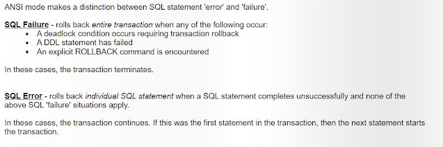


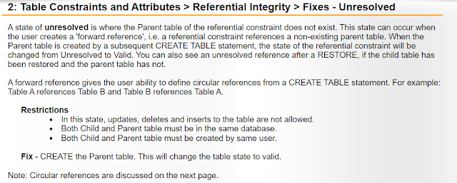


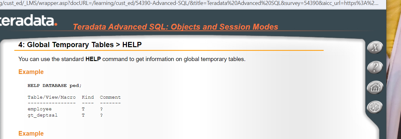


Comments
Post a Comment